In 1936, a German physician and philosopher named Paul Lueg received U.S. Patent 2,043,416 for a concept that would take nearly 60 years to reach consumers. His invention: using sound to cancel sound. The patent described how to attenuate sinusoidal tones in ducts by phase-advancing the acoustic wave and canceling arbitrary sounds around a loudspeaker by inverting polarity. Lueg had discovered the fundamental principle of active noise control. He had no way to implement it.
The problem wasn’t the physics—it was the speed. Lueg’s concept required measuring incoming sound, computing an inverted waveform, and playing it back through a speaker. All of this needed to happen faster than sound could travel from the microphone to the listener’s ear. In 1936, analog electronics were simply too slow. The idea remained a theoretical curiosity for two decades.
Today, active noise cancellation (ANC) is ubiquitous. Noise-canceling headphones are a multi-billion dollar market. Automotive manufacturers install ANC systems in vehicle cabins. Aircraft manufacturers use the technology to reduce cabin noise. Yet the fundamental constraints that challenged Lueg remain: sound travels at approximately 343 meters per second, and the anti-noise must arrive at precisely the right moment to cancel it.
The Physics of Destructive Interference
Sound is a pressure wave—a propagating disturbance in air molecules that alternates between compression (high pressure) and rarefaction (low pressure). When two sound waves occupy the same space, they superimpose: their pressures add algebraically. This principle, called superposition, is the foundation of all active noise control.
Consider two identical sine waves. If they align perfectly—with crest matching crest and trough matching trough—they add constructively, doubling the amplitude. But if one wave is shifted by exactly half a wavelength (180 degrees), the crest of one aligns with the trough of the other. They add destructively, summing to zero.
$$p_{total}(t) = p_1(t) + p_2(t) = A\sin(\omega t) + A\sin(\omega t + \pi) = 0$$This mathematical ideal—perfect cancellation—is what ANC systems attempt to achieve. The challenge is that real noise is not a single sine wave. It’s a complex waveform containing many frequencies, constantly changing, arriving from multiple directions, and reflecting off surfaces.
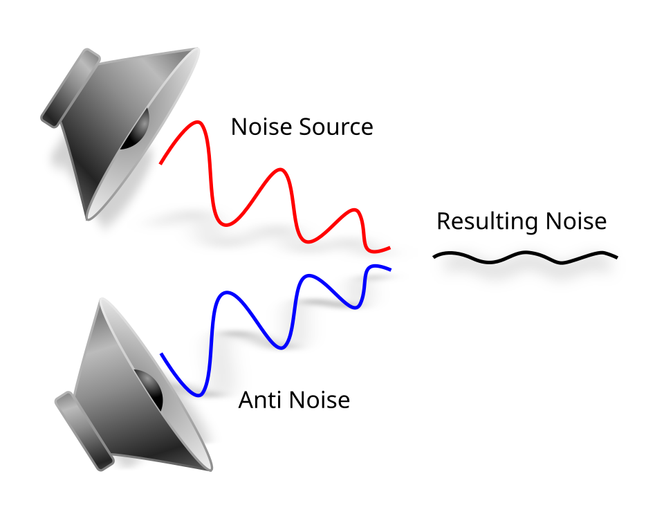
Image source: Wikipedia - Active Noise Control
The diagram above illustrates the core principle: an unwanted primary noise is measured, inverted, and combined with the original to produce silence at the listener’s position.
Why ANC Works for Low Frequencies Only
Walk into any coffee shop wearing noise-canceling headphones. The low drone of the espresso machine, the rumble of traffic outside, the thrum of the HVAC system—all noticeably reduced. But the barista calling out orders? A child crying at a nearby table? Your phone conversation? These remain clearly audible.
The reason lies in wavelength and timing. Sound wavelength is inversely proportional to frequency:
$$\lambda = \frac{c}{f}$$Where $\lambda$ is wavelength, $c$ is the speed of sound (approximately 343 m/s at room temperature), and $f$ is frequency. At 100 Hz, the wavelength is about 3.43 meters. At 1,000 Hz, it’s 34.3 centimeters. At 4,000 Hz—roughly the frequency of a baby’s cry—it’s just 8.6 centimeters.
For effective cancellation, the anti-noise must arrive at the listener’s ear within a small fraction of a wavelength from the optimal phase. A phase error of just 90 degrees—a quarter wavelength—reduces the cancellation from total to merely 3 dB (half the amplitude). At 100 Hz, a quarter wavelength is about 86 centimeters; sound travels this distance in roughly 2.5 milliseconds. The ANC system has comfortable margins.
At 4,000 Hz, a quarter wavelength is just 2.15 centimeters. Sound travels this distance in about 63 microseconds. The ANC system must measure the incoming sound, compute the anti-noise, and play it back in less than the time between two samples at typical audio rates (about 21 microseconds at 48 kHz sampling). Any processing delay, any latency in the electronics, destroys the cancellation.
graph LR
    A[Incoming Noise] --> B[Microphone]
    B --> C[ADC<br/>~10-20 μs]
    C --> D[DSP Processing<br/>~10-50 μs]
    D --> E[DAC<br/>~10-20 μs]
    E --> F[Speaker<br/>~5-10 μs]
    F --> G[Anti-Noise<br/>at Ear]

    H[Total Latency<br/>~35-100 μs] --> I{Phase Match?}
    I -->|< 1/4 wavelength| J[Effective Cancellation]
    I -->|> 1/4 wavelength| K[Degraded Performance]

    style H fill:#ff9999
    style J fill:#99ff99
    style K fill:#ffff99
The diagram above shows the latency budget for an ANC system and how it relates to cancellation effectiveness. Every microsecond counts at high frequencies.
Research published in technical literature confirms this limitation: ANC is most effective below 1,000 Hz, with performance degrading rapidly above that threshold. The wavelength becomes shorter than practical microphone-to-speaker distances, and processing delays introduce phase errors that prevent effective cancellation.
The Secondary Path Problem
Lueg’s original patent assumed the anti-noise would simply be played through a speaker. Reality is more complicated. The electrical signal from the ANC controller must travel through a DAC, an amplifier, and a speaker before becoming acoustic energy. The resulting sound then propagates through air to reach the error microphone and the listener’s ear. This entire chain—the electro-acoustic path from controller output to the point where cancellation is desired—is called the secondary path.
The secondary path introduces three critical effects:
- Delay: Sound takes time to travel from speaker to ear
- Frequency response: Speakers and microphones have non-flat responses
- Phase shift: The signal is delayed differently at different frequencies
If the ANC controller generates the exact inverse of the incoming noise, but the secondary path delays it by 2 milliseconds, the anti-noise arrives at the wrong time. Instead of cancellation, you get interference patterns—some frequencies cancel, others add.
This is why modern ANC systems must model the secondary path. Before the system can effectively cancel noise, it must understand how its own speaker output transforms before reaching the listener. The standard approach uses an adaptive filter to estimate this transfer function, typically by playing a calibration signal through the speaker and measuring the result at the error microphone.
Three Architectures: Feedforward, Feedback, and Hybrid
Modern ANC systems use one of three fundamental architectures, each with distinct advantages and limitations.
Feedforward ANC
In feedforward systems, a reference microphone is positioned upstream from the noise source or outside the ear cup. This microphone captures the incoming noise before it reaches the listener, giving the system time to compute and play the anti-noise.
The advantage is predictability: the system knows what’s coming. The disadvantage is acoustic feedback—the speaker’s output can be picked up by the reference microphone, creating a feedback loop. Additionally, the reference microphone must be positioned where it captures noise before it reaches the listener, which isn’t always practical.
Feedback ANC
Feedback systems eliminate the reference microphone entirely. They use only an error microphone positioned at the point where cancellation is desired. The controller observes the residual noise at this point and continuously adjusts its output to minimize it.
The advantage is simplicity—no reference microphone needed. The disadvantage is that feedback systems can only cancel noise that’s predictable from past samples. They work well for steady-state or slowly varying sounds but struggle with sudden transients.
Hybrid ANC
Hybrid systems combine both approaches, using a reference microphone for feedforward cancellation and an error microphone for feedback correction. This provides the best of both worlds: good performance on both predictable and unpredictable noise sources.
Most high-end noise-canceling headphones use hybrid architecture. The reference microphone on the outside of the ear cup captures incoming noise, while the error microphone inside the ear cup measures residual sound and provides feedback correction.
flowchart TB
    subgraph Feedforward["Feedforward Path"]
        FF_Ref[Reference Microphone<br/>Outside Ear Cup]
        FF_DSP[DSP Controller]
        FF_Spk[Speaker]
    end

    subgraph Feedback["Feedback Path"]
        FB_Err[Error Microphone<br/>Inside Ear Cup]
        FB_DSP[Adaptive Filter]
    end

    Noise[Incoming Noise] --> FF_Ref
    FF_Ref --> FF_DSP
    FF_DSP --> FF_Spk
    FF_Spk --> AntiNoise[Anti-Noise]

    AntiNoise --> FB_Err
    FB_Err --> FB_DSP
    FB_DSP --> FF_DSP

    style Feedforward fill:#e1f5fe
    style Feedback fill:#fff3e0
The diagram above shows how feedforward and feedback paths combine in a hybrid system, with each contributing to the final anti-noise signal.
The FxLMS Algorithm: Making ANC Adaptive
Early ANC systems used fixed filters designed for specific noise spectra. They worked well in controlled environments but failed when noise characteristics changed. The solution came from adaptive signal processing: the filtered-x least mean square (FxLMS) algorithm.
The LMS algorithm, developed by Bernard Widrow in the 1950s, continuously adjusts filter coefficients to minimize an error signal. For ANC, the error signal is the residual noise measured at the error microphone. The goal is to drive this error to zero.
Standard LMS cannot be directly applied to ANC because of the secondary path. The filter output doesn’t immediately affect the error signal—it must first pass through the speaker, the acoustic path, and the microphone. This delay violates the assumptions of the standard LMS algorithm.
FxLMS solves this by filtering the reference signal through an estimate of the secondary path before using it in the coefficient update equation:
$$w(n+1) = w(n) + \mu e(n) x'(n)$$Where $w(n)$ is the filter coefficient vector, $\mu$ is the step size (learning rate), $e(n)$ is the error signal, and $x'(n)$ is the reference signal filtered through the secondary path estimate.
The step size $\mu$ controls the trade-off between convergence speed and steady-state performance. Larger step sizes cause faster adaptation but may prevent the filter from settling to the optimal solution. The maximum stable step size depends on the secondary path response, the filter length, and the input signal characteristics:
$$\mu_{max} = \frac{2}{\|s\|^2 \sigma_x^2 (L + 2D_{eq})}$$Where $\|s\|^2$ is the squared norm of the secondary path impulse response, $\sigma_x^2$ is the reference signal power, $L$ is the filter length, and $D_{eq}$ is the secondary path equivalent delay.
Research from the University of Auckland, published in Signal Processing journal, derived this expression for general secondary paths—extending earlier work that had only considered pure delay cases.
Real-World Performance Measurements
A study published in The Hearing Review measured the actual attenuation provided by noise-canceling headphones in a controlled environment. Using 85 dBA of white noise, researchers measured sound pressure levels inside participants’ ear canals with and without active noise cancellation engaged.
The results showed approximately 13 dB of noise reduction. This is significant—13 dB represents roughly a 95% reduction in acoustic power—but far from total silence. The attenuation was most effective at frequencies below 1,000 Hz, consistent with the theoretical limitations discussed earlier.
Other studies have found similar results. A feasibility study published in Applied Acoustics in 2026 reported ANC systems reducing background noise by up to 20 dB at low frequencies, with greater reduction for pure tones than for broadband noise.
The Hyundai Motor Group’s Road-noise Active Noise Control (RANC) system, introduced in 2019, represents one of the most ambitious automotive applications. The system uses acceleration sensors to detect road vibrations, processes the signal through a digital signal processor, and generates anti-noise through the vehicle’s audio system. Hyundai reports achieving 3 dB of cabin noise reduction—which represents approximately a 50% reduction in perceived loudness.

Image source: Hyundai Motor Group - RANC Technology
The Hyundai RANC diagram illustrates the complete signal chain: road vibration is detected by acceleration sensors, processed by the DSP, and converted to anti-noise played through the vehicle’s speakers, with microphones monitoring the residual noise for feedback.
The Latency Race
Every component in the ANC signal chain adds latency:
- Microphone transduction: Converting acoustic pressure to electrical signal (typically microseconds)
- Anti-aliasing filter: Removing frequencies above Nyquist before sampling (typically a few samples)
- Analog-to-digital conversion: Typically 10-20 microseconds for audio-grade ADCs
- DSP processing: The algorithm itself, typically 10-50 microseconds for simple FxLMS
- Digital-to-analog conversion: Similar to ADC
- Amplifier: Usually negligible for modern Class-D designs
- Speaker transduction: Converting electrical signal back to acoustic pressure (microseconds)
- Acoustic propagation: Sound traveling from speaker to ear (roughly 3 milliseconds per meter)
For headphones, the acoustic path from speaker to ear is very short—centimeters. This leaves a latency budget of tens of microseconds. Modern ANC chips from companies like Qualcomm, MediaTek, and others achieve total latencies in the 20-40 microsecond range for the entire processing chain.
For automotive applications, the distances are larger, but so is the available processing time. The Hyundai RANC system processes road noise in approximately 2 milliseconds—fast enough to generate anti-noise before road vibrations reach the cabin.
Why Your Headphones Can’t Cancel Everything
Understanding the physics and engineering of ANC reveals why certain sounds resist cancellation:
High-frequency sounds: Wavelengths become shorter than practical microphone-to-speaker distances. A 10 kHz tone has a wavelength of just 3.4 centimeters. The phase varies significantly across the ear cup, making single-point cancellation ineffective.
Sudden transients: A hand clap, a dropped object, a shout—these sounds have rapid onsets that leave little time for the ANC system to respond. Feedback architectures particularly struggle with transients.
Near-field sources: Sounds coming from very close to the ear arrive at the outer microphone and ear canal nearly simultaneously, leaving no processing time.
Complex multi-source environments: In a room with multiple noise sources at different locations, generating a single anti-noise signal that cancels all of them simultaneously is mathematically impossible.
Speech and music: These contain broad frequency content extending well above 1 kHz. ANC may reduce the low-frequency components but leaves the essential character of these sounds intact—which is usually considered a feature, not a bug.
Beyond Headphones: Industrial and Automotive Applications
While consumer headphones represent the most visible application of ANC, the technology has found uses in more demanding environments.
Aircraft cabins: Propeller-driven aircraft generate strong low-frequency noise from the propeller blade passage rate. ANC systems installed in cabin headrests can reduce this noise by 6-10 dB, improving passenger comfort without adding weight. Research on the BAe HS.748 aircraft demonstrated successful blade-pass noise reduction using multi-channel ANC.
Automotive cabins: Engine harmonics, road noise, and tire cavity resonances all fall in the frequency range where ANC is effective. Modern vehicles increasingly integrate ANC into the audio system, using existing speakers to generate anti-noise.
Industrial ducts: HVAC systems generate significant low-frequency noise that propagates through ductwork. ANC can reduce this noise at the duct outlet without the pressure drop associated with passive silencers.
Medical devices: MRI machines produce extremely loud acoustic noise from gradient coil vibration. ANC systems can reduce patient exposure, improving the examination experience.
The Future: Lower Latency, Higher Frequencies
The trajectory of ANC development follows the trajectory of computing: faster processors, lower latency, better algorithms.
Neural network-based approaches are beginning to appear in research literature. A 2025 paper from NVIDIA demonstrated deep learning models achieving comparable or better noise reduction than traditional FxLMS while handling non-stationary noise sources more effectively. The challenge is computational: neural networks typically require more processing than the elegant simplicity of FxLMS.
Hardware improvements continue to push latency lower. New ADC and DAC architectures, faster DSP cores, and optimized signal paths are gradually extending the effective frequency range upward. Current high-end ANC headphones show measurable cancellation up to about 2 kHz—a significant improvement over systems from a decade ago.
The fundamental physics remains: wavelength determines what’s possible. No amount of processing speed can change the speed of sound. But within those physical constraints, the technology continues to advance toward the ideal that Paul Lueg imagined in 1936: using sound itself to create silence.
References
-
Lueg, P. (1936). Process of silencing sound oscillations. U.S. Patent 2,043,416.
-
Widrow, B., et al. (1975). Adaptive noise cancelling: Principles and applications. Proceedings of the IEEE, 63(12), 1692-1716.
-
Kuo, S. M., & Morgan, D. R. (1996). Active Noise Control Systems: Algorithms and DSP Implementations. Wiley-Interscience.
-
Elliott, S. J. (2001). Signal Processing for Active Control. Academic Press.
-
Ardekani, I. T., & Abdulla, W. H. (2010). Theoretical convergence analysis of FxLMS algorithm. Signal Processing, 90(12), 3046-3055.
-
Ardekani, I. T., & Abdulla, W. H. (2011). On the convergence of real-time active noise control systems. Signal Processing, 91(5), 1262-1274.
-
Baur, F. X., & Zalewski, T. R. (2008). Attenuation values of a noise-cancelling headphone. The Hearing Review.
-
Hyundai Motor Group. (2019). Hyundai’s World’s First Road-Noise Active Noise Control, RANC. https://www.hyundaimotorgroup.com/en/story/CONT0000000000090151
-
MathWorks. (2024). Active Noise Control with Simulink Real-Time. https://www.mathworks.com/help/audio/ug/active-noise-control-with-simulink.html
-
Fiveable. (2024). Limitations and challenges of active noise control. https://fiveable.me/noise-control-engineering/unit-10/limitations-challenges-active-noise-control/
-
Wikipedia. (2024). Active noise control. https://en.wikipedia.org/wiki/Active_noise_control
-
Morgan, D. R. (1980). An analysis of multiple correlation cancellation loops with a filter in the auxiliary path. IEEE International Conference on ICASSP ‘80, 457-461.
-
Burgess, J. C. (1981). Active adaptive sound control in a duct: Computer simulation. Journal of the Acoustical Society of America, 70, 715-726.
-
Eriksson, L. J. (1991). Recursive algorithms for active noise control. International Symposium of Active Control of Sound and Vibration, 137-146.
-
Fogel, L. J. (1958). Methods of improving intelligence under random noise interference. U.S. Patent 2,866,848.
-
Olson, H. F. (1956). Electronic control of noise, vibration and reverberation. Journal of the Acoustical Society of America, 28, 966-972.