How Bloom Filters Store 100 Million Items in 120 MB While Never Missing a Match

In 1970, Burton Howard Bloom faced a problem that would feel familiar to any modern software engineer working with large datasets. He needed to check whether words required special hyphenation rules, but storing 500,000 dictionary entries in memory was prohibitively expensive. His solution—a data structure that uses dramatically less space than any traditional approach—became one of the most widely deployed probabilistic data structures in computing history.

The insight was radical: what if you could trade certainty for space? A Bloom filter will never tell you an item is absent when it’s actually present (no false negatives), but it might occasionally claim an item exists when it doesn’t (false positives). For many applications, this trade-off is not just acceptable—it’s transformative.

The Mathematics of Space Efficiency

A Bloom filter consists of two components: a bit array of size m and k independent hash functions. To add an element, you run it through all k hash functions and set the corresponding bits to 1. To check membership, you hash the element and verify all resulting positions contain 1.

The false positive probability follows from basic probability theory. After inserting n elements, the probability that a specific bit remains 0 is:

For a query element not in the set, all k bits must be 1, giving a false positive probability of:

The optimal number of hash functions that minimizes this probability is:

This yields a remarkably clean result: for a desired false positive rate ε, you need approximately $-\log_2(\epsilon)$ bits per element. Want a 1% false positive rate? That’s roughly 9.6 bits per element. A 0.1% rate needs about 14.4 bits.

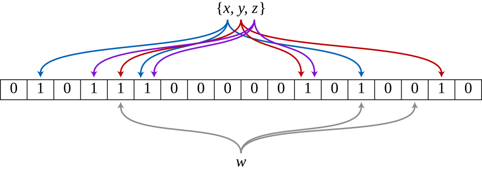
Image source: Wikimedia Commons

To put this in concrete terms: storing 100 million URLs with a 1% false positive rate requires approximately 120 MB. A traditional hash set storing even just 64-bit hashes would need 800 MB. The Bloom filter achieves roughly 7× space savings—and the savings grow as the elements themselves become larger.

The Hash Function Question

Early implementations believed you needed k independent hash functions. This seemed computationally expensive, leading many to avoid Bloom filters for query-intensive workloads.

In 2006, Kirsch and Mitzenmacher published a result that changed this assumption entirely. They proved that you only need two hash functions, h₁(x) and h₂(x), to simulate k functions using the formula:

This “double hashing” approach produces the same asymptotic false positive probability as using k truly independent hash functions. The insight comes from the hashing literature—Knuth had described similar techniques for open addressing—but Kirsch and Mitzenmacher proved it applies to Bloom filters without performance degradation.

Image source: Wikimedia Commons

Where Bloom Filters Shine

The Akamai content delivery network discovered that approximately 75% of web objects in their caches were “one-hit-wonders”—requested exactly once and never again. Storing these wasted disk space and write bandwidth. Their solution: maintain a Bloom filter of all requested URLs, and only cache an object on its second request. This dramatically reduced disk writes while increasing cache hit rates for genuinely popular content.

Distributed databases face a different challenge. When a read request arrives, the system must determine which nodes might contain the requested data. Google Bigtable, Apache HBase, and Cassandra all use Bloom filters to avoid expensive disk seeks for non-existent rows. A Bloom filter can fit in memory and quickly eliminate the vast majority of unnecessary I/O operations.

PostgreSQL implements Bloom filters as an index access method. Rather than creating multiple indexes on different columns, a single Bloom index can handle multi-column equality queries. The trade-off is approximate results, but for many analytical workloads, the space savings justify occasional false positives.

Web browsers have used Bloom filters for safe-browsing checks. Rather than maintaining a complete local database of malicious URLs—impractical due to size—Chrome previously shipped a Bloom filter that could quickly determine when a URL was definitely safe. Only when the filter returned “possibly malicious” did it contact Google’s servers for verification.

The Deletion Problem and Its Solutions

Classic Bloom filters have a fundamental limitation: you cannot delete elements. When you set bits during insertion, multiple elements might share the same bit positions. Clearing a bit to “remove” one element could silently corrupt the filter for others.

Counting Bloom Filters address this by replacing single bits with small counters (typically 3-4 bits). Insertion increments counters; deletion decrements them. This solves the deletion problem but increases space usage by 3-4×, eliminating much of the space advantage.

Image source: Wikimedia Commons

Cuckoo filters, introduced by Fan, Andersen, Kaminsky, and Mitzenmacher in 2014, offer an alternative approach. They store fingerprints in a compact hash table structure inspired by cuckoo hashing. The key advantages: deletion is supported, they often use less space than Bloom filters for the same false positive rate, and lookups can terminate early upon a match. However, construction can fail if the table becomes too full, and performance degrades with high load factors.

When Not to Use Bloom Filters

Bloom filters excel when false positives are cheap but false negatives are catastrophic. The CDN caching use case perfectly illustrates this: a false positive means caching an extra item (minor cost), while a false negative means not caching something popular (significant cost).

They’re inappropriate when:

• You need exact membership testing (use a hash set)
• The set is small enough that space savings don’t matter
• You need to enumerate the elements (Bloom filters can’t retrieve stored items)
• Deletion is frequent and space is tight (consider Cuckoo filters or quotient filters)
• Elements are small and numerous enough that a simple bit array suffices

The theoretical minimum space for any approximate membership data structure is approximately $n \log_2(1/\epsilon)$ bits. Bloom filters use about 44% more space than this theoretical optimum. For applications where absolute space efficiency matters, quotient filters and xor filters approach this bound more closely—though with increased complexity and reduced flexibility.

Implementation Considerations

The quality of hash functions matters less than intuition suggests. Non-cryptographic hashes like MurmurHash, xxHash, or FNV work well. What matters more is that the hashes appear independent; using different seeds or offsets with the same hash function family is sufficient.

Memory access patterns affect performance significantly. For large filters, the k random memory accesses during lookup can cause cache misses. Some implementations group hash outputs into cache-line-sized blocks to improve locality, though this typically increases space usage.

The filter’s fill ratio—the fraction of bits set to 1—provides a health check. A well-tuned filter should have approximately half its bits set. If nearly all bits are 1, the false positive rate will be much higher than expected. If few bits are set, you’re wasting space.

The Legacy

Bloom’s original paper solved a hyphenation problem that few encounter today. But the core insight—that accepting controlled uncertainty enables dramatic efficiency gains—has proven remarkably durable. From blockchain synchronization to network routing to database query optimization, the humble Bloom filter quietly underpins systems that process billions of operations daily.

The next time your database query completes in milliseconds rather than seconds, or a web page loads from cache instead of origin, a Bloom filter may have been the invisible enabler. Not bad for a data structure invented to hyphenate words.