In 1996, Patrick O’Neil and his colleagues at the University of Massachusetts Boston published a paper describing a data structure that would take nearly a decade to find widespread adoption. The Log-Structured Merge-Tree (LSM-Tree) was designed to solve a problem that barely existed at the time: how to efficiently index data when writes vastly outnumber reads.
Today, LSM-Trees power the storage engines of Cassandra, RocksDB, LevelDB, HBase, InfluxDB, and countless other systems that handle massive write throughput. Yet the fundamental insight remains surprisingly misunderstood: LSM-Trees don’t just “write faster”—they fundamentally restructure how data moves from memory to disk.
The B-Tree Problem: Why Random Writes Kill Performance
Traditional databases built on B+ trees face an unavoidable physical constraint. When you update a record, the database must find its location on disk and modify that exact location. On a spinning hard drive, this means moving the read head to the correct cylinder, waiting for the platter to rotate, and then performing the write. Even on SSDs, random writes incur significant overhead because flash memory must be erased before being rewritten at the page level.
Consider what happens when you insert 1 million records into a B+ tree. Each insertion potentially requires:
- Traversing the tree to find the correct leaf node
- Reading that node from disk (if not cached)
- Modifying the node
- Writing it back to the same location
If the tree has depth 4 and nodes aren’t cached, that’s potentially 4 disk reads and 1 disk write per insertion. At 10ms per random disk operation on an HDD, you’re looking at 50ms per write—20 writes per second. Even with SSDs reducing this to 0.1ms per operation, you’re still limited by the random I/O pattern.
The LSM-Tree inverts this problem entirely.
The Architecture: Memory First, Disk Later
An LSM-Tree consists of multiple components arranged in a hierarchy. At the top sits an in-memory structure called the memtable—typically implemented as a skip list, red-black tree, or similar ordered data structure. Below it are multiple levels of on-disk files called SSTables (Sorted String Tables).

Image source: Wikipedia - Log-structured merge-tree
The Write Path: Sequential by Design
When a write arrives, the system:
- Appends the operation to a Write-Ahead Log (WAL) for durability
- Inserts the key-value pair into the memtable
That’s it. No disk seeks, no random writes, no tree rebalancing. The write hits memory immediately, and the WAL append is sequential—exactly what both HDDs and SSDs handle efficiently.
When the memtable reaches a configured size threshold (typically 64-256 MB in RocksDB), it becomes immutable, a new memtable takes its place, and a background thread flushes the old memtable to disk as an SSTable. This flush is a pure sequential write: iterate through the sorted memtable and write entries in order.
flowchart TB
    subgraph Write["Write Path"]
        W[Write Request] --> WAL[Append to WAL]
        WAL --> MT[Insert to Memtable]
        MT --> |Size Threshold| IMT[Mark Immutable]
        IMT --> |Background Flush| SST[Write SSTable]
    end
The Read Path: The Trade-off
Reads work differently. To find a key, the system must check:
- The active memtable
- Any immutable memtables awaiting flush
- SSTables from newest to oldest
Each SSTable is sorted, enabling binary search within the file. But in the worst case, a read might need to check multiple SSTables across multiple levels before finding the key—or concluding it doesn’t exist.
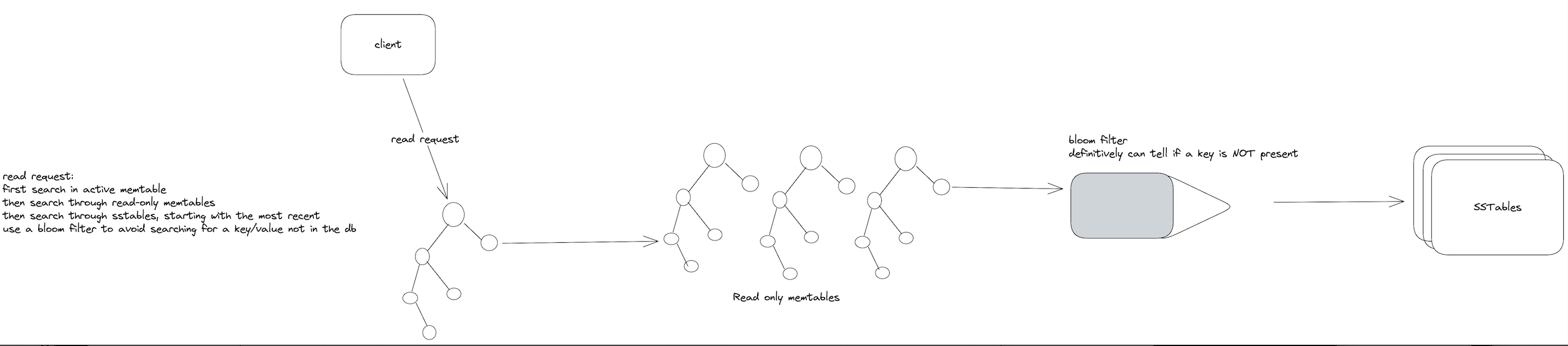
Image source: David Archuleta Jr. - LSM Trees Introduction
This is where Bloom filters become essential. Each SSTable maintains a Bloom filter in memory—a probabilistic data structure that can definitively answer “this key is NOT in this SSTable” without touching the disk. With a 1% false positive rate, Bloom filters eliminate roughly 99% of unnecessary disk reads for non-existent keys.
SSTable Structure: More Than Just Sorted Files
An SSTable isn’t simply a list of key-value pairs. Modern implementations like RocksDB organize SSTables into:
- Data blocks: Compressed groups of key-value pairs (typically 4-64 KB each)
- Index block: A sparse index mapping key ranges to data block offsets
- Filter block: The Bloom filter for this SSTable
- Footer: Metadata including checksums and block locations
Within each data block, keys often share prefixes. If one key is user:1001:email and the next is user:1001:name, the SSTable can encode this as [length of shared prefix][suffix][value], dramatically reducing storage for hierarchical keys.
Compression algorithms like LZ4, Snappy, or Zstd are applied per-block. LZ4 decompresses at memory bandwidth speeds (multiple GB/s), making it effectively free for reads while saving 2-5× storage space.
Levels and Compaction: The Hidden Cost
The defining characteristic of an LSM-Tree is compaction—the process of merging multiple SSTables into fewer, larger ones. This is where the “merge” in LSM-Tree becomes apparent.
Leveled Compaction
Used by RocksDB and LevelDB, leveled compaction organizes SSTables into levels with exponentially increasing sizes:
- Level 0: SSTables directly flushed from memtables. Keys may overlap between files.
- Level 1: Size $\approx$ 10× Level 0. SSTables have non-overlapping key ranges.
- Level 2: Size $\approx$ 10× Level 1. And so on…
When Level $L$ exceeds its size limit, the system selects one SSTable from Level $L$ and merges it with all overlapping SSTables from Level $L+1$. This is a merge-sort operation: read all input SSTables, write a new sorted SSTable to Level $L+1$.
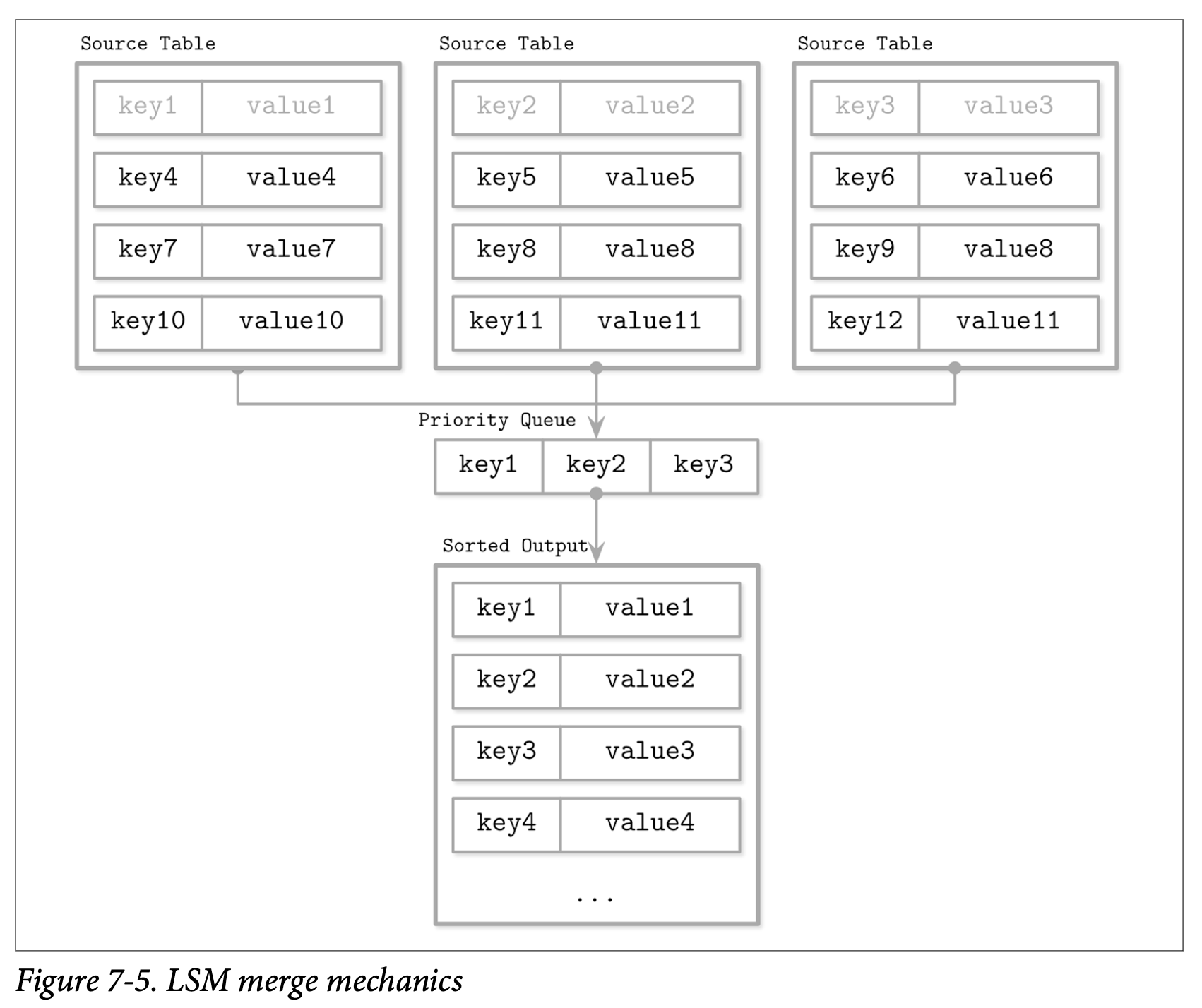
Image source: David Archuleta Jr. - LSM Trees Introduction
Size-Tiered Compaction
Used by Cassandra, size-tiered compaction groups SSTables by size rather than enforcing non-overlapping key ranges. When enough SSTables of similar size accumulate, they’re merged into a single larger SSTable.
This approach is simpler and works well for write-heavy workloads, but can lead to higher read amplification since multiple SSTables at the same level might contain overlapping keys.
Tiered Compaction
A hybrid approach that uses size-tiered merging for smaller levels and leveled merging for larger levels. RocksDB implements this as “tiered+leveled” compaction, aiming to minimize write amplification on smaller levels while keeping read amplification low on larger levels.
The Mathematics of Amplification
Three metrics define LSM-Tree performance:
Write Amplification
The ratio of bytes written to disk versus bytes written by the application. In leveled compaction with size ratio $T$ (typically 10):
$$WA \approx T \cdot \log_T(N/B)$$Where $N$ is database size and $B$ is the size of a memtable flush. For a 1 TB database with 64 MB memtables and $T=10$, write amplification is approximately 50—every 1 byte you write causes 50 bytes of disk writes through compaction.
Read Amplification
The number of disk reads required for a point query. Without Bloom filters:
$$RA = O\left(\frac{\log^2(N/B)}{\log T}\right)$$With Bloom filters of total size $M$ for $N$ keys, point lookups for non-existent keys drop to approximately $O(N/M)$—essentially constant for well-tuned filters.
Space Amplification
The ratio of on-disk size versus logical data size. For leveled compaction:
$$SA \approx 1 + \frac{1}{T}$$With $T=10$, space amplification is approximately 1.1—the database uses about 10% more space than the logical data size.
Deletions: The Tombstone Problem
LSM-Trees don’t delete data immediately. When you delete a key, the system writes a tombstone—a special marker indicating the key has been deleted. The tombstone lives in the memtable, gets flushed to an SSTable, and only disappears during compaction when it merges with the SSTable containing the deleted key.
This creates two issues:
- Space overhead: Deleted data persists until compaction reaches it
- Read overhead: A read must process tombstones to know a key doesn’t exist
Cassandra famously suffered from “tombstone overwhelm” where heavy delete workloads could cause reads to time out because they had to process millions of tombstones. Modern implementations use tombstone garbage collection strategies to address this.
Range Queries: Strength and Weakness
LSM-Trees handle range queries differently than B+ trees. For a range query, the system must:
- Start iterators at the range start in each relevant SSTable
- Merge these iterators using a priority queue
- Return results until the range end
For short ranges (fewer keys than twice the number of levels), cost is proportional to the number of levels. For long ranges, cost is dominated by the largest level containing most data.
xychart-beta
    title "LSM Tree vs B+ Tree: Range Query Performance"
    x-axis ["10 keys", "100 keys", "1000 keys", "10000 keys", "100000 keys"]
    y-axis "Disk Reads" 0 --> 2000
    bar [15, 50, 150, 500, 1500]
    line [4, 4, 15, 120, 1200]
The chart illustrates that B+ trees excel at short range queries (single leaf node traversal), while LSM-Trees catch up for longer scans where sequential reads dominate.
Real-World Implementations
LevelDB: The Minimalist Pioneer
Created by Jeff Dean and Sanjay Ghemawat at Google in 2011, LevelDB extracted the tablet storage engine from Bigtable into a standalone library. It established the modern LSM-Tree pattern: skip list memtable, sorted SSTables, leveled compaction. Its simplicity (roughly 20,000 lines of C++) makes it ideal for embedded use cases like Chrome’s IndexedDB backend.
RocksDB: The Performance Beast
Facebook forked LevelDB in 2012 and transformed it into RocksDB, optimizing for flash storage and multi-core CPUs. Key enhancements include:
- Multi-threaded compaction: Parallel merge operations across CPU cores
- Prefix bloom filters: Optimized for hierarchical keys like
user:ID:field - Column families: Multiple logical databases in one physical instance
- Dynamic level sizing: Adapts to workload patterns
RocksDB achieves millions of writes per second on modern NVMe SSDs—far beyond what B+ tree databases can match.
Cassandra: Distributed Scale
Apache Cassandra uses size-tiered compaction by default, with SSTables distributed across a ring of nodes. Each node handles a token range, and writes are replicated across multiple nodes for fault tolerance. Cassandra’s compaction strategies have evolved significantly:
- SizeTieredCompactionStrategy: Default, good for write-heavy workloads
- LeveledCompactionStrategy: Better read performance, higher write amplification
- DateTieredCompactionStrategy: Optimized for time-series data
When LSM-Trees Win (and When They Don’t)
LSM-Trees Excel When:
- Write throughput is critical: Sequential writes beat random writes by 10-100×
- Data size exceeds memory: The tiered approach naturally handles large datasets
- Time-series or append-heavy workloads: New data flows to the top levels naturally
- SSD storage: Flash benefits enormously from reduced write amplification
B+ Trees Remain Better When:
- Read-heavy workloads: Single-tree traversal beats multi-level search
- Strong consistency requirements: In-place updates simplify transaction handling
- Predictable latency: No compaction spikes
- Small datasets fitting in memory: The LSM advantage disappears
A 2022 USENIX paper revisiting B+ trees versus LSM-Trees on modern hardware found that the crossover point for write throughput occurs around 50,000 writes per second for typical configurations. Below that threshold, B+ trees often win on overall performance. Above it, LSM-Trees dominate.
The Hidden Complexity
LSM-Trees aren’t a free lunch. The performance gains come with operational complexity:
Compaction tuning: The size ratio, level sizes, and compaction threads all affect the write/read/space amplification trade-offs. A misconfigured system can suffer from write stalls when compaction can’t keep up.
Read latency variance: While write latency is consistently low, read latency varies wildly. A cache miss on a key in a deep level can take milliseconds, while a memtable hit returns in microseconds.
Memory pressure: Bloom filters, block caches, and memtables all compete for memory. Under-provisioning any of these degrades performance significantly.
Background I/O: Compaction consumes disk bandwidth. On saturated systems, this can compete with foreground operations, causing latency spikes.
Looking Forward
The LSM-Tree continues evolving. Recent research has produced:
- WiscKey: Separates keys and values to reduce write amplification for large values
- PebblesDB: Fragmented LSM-Trees that reduce write amplification by allowing key overlap within levels
- Monkey: Optimal Bloom filter allocation across levels
- REMIX: Efficient range queries through reordering indices
These optimizations address specific weaknesses while preserving the fundamental write-optimized architecture that made LSM-Trees successful.
References
-
O’Neil, P., Cheng, E., Gawlick, D., & O’Neil, E. (1996). “The Log-Structured Merge-Tree (LSM-Tree).” Acta Informatica, 33(4), 351-385.
-
Dean, J., & Ghemawat, S. (2011). “LevelDB: A Fast Persistent Key-Value Store.” Google Open Source Blog.
-
Chang, F., et al. (2006). “Bigtable: A Distributed Storage System for Structured Data.” OSDI ‘06.
-
Sarkar, S., et al. (2021). “Constructing and Analyzing the LSM Compaction Design Space.” VLDB Endowment, 14, 2216-2230.
-
Dayan, N., & Idreos, S. (2018). “PebblesDB: Building Key-Value Stores using Fragmented Log-Structured Merge Trees.” SIGMOD ‘18.
-
Luo, C., & Carey, M. J. (2020). “LSM-based Storage Techniques: A Survey.” The VLDB Journal, 29, 393-418.
-
Facebook Inc. “RocksDB Wiki.” GitHub Repository.
-
Apache Cassandra Documentation. “Storage Engine Architecture.”
-
TiKV Deep Dive. “B-Tree vs LSM-Tree.” tikv.org.
-
Petrov, A. (2019). “Database Internals: A Deep Dive into How Distributed Data Systems Work.” O’Reilly Media.