In 1987, three researchers at the University of California, Berkeley published a paper that would fundamentally change how we think about data storage. David Patterson, Garth Gibson, and Randy Katz proposed something counterintuitive: instead of buying one expensive, reliable disk drive, why not combine many cheap, unreliable ones into a system more reliable than any single drive could ever be? They called it RAID—Redundant Arrays of Inexpensive Disks.
The insight was mathematical, not magical. By distributing data across multiple drives with carefully calculated redundancy, you could achieve both performance and reliability that would be impossible with a single disk. The key was a simple operation that most programmers learn in their first computer science course: XOR.
The XOR Foundation: How Parity Actually Works
At the heart of RAID’s data protection lies the exclusive OR operation. XOR is a binary operation that outputs 1 only when its inputs differ. The truth table is straightforward:
| Input A | Input B | Result |
|---|---|---|
| 0 | 0 | 0 |
| 0 | 1 | 1 |
| 1 | 0 | 1 |
| 1 | 1 | 0 |
What makes XOR remarkable for storage is its self-inverting property. If A XOR B = P, then:
- A XOR P = B
- B XOR P = A
This creates a mathematical relationship where any one value can be reconstructed from the other two. RAID exploits this property at scale.
Consider a simplified example with three disks. Suppose we want to store the character ‘a’ (ASCII 97, binary 01100001) on Disk 1 and ‘b’ (ASCII 98, binary 01100010) on Disk 2. The parity is calculated as:
  01100001 (a)
XOR 01100010 (b)
  = 00000011 (parity = 3)
This parity value (3) gets stored on Disk 3. If Disk 1 fails, we can reconstruct ‘a’ by XORing what remains:
  01100010 (b from Disk 2)
XOR 00000011 (parity from Disk 3)
  = 01100001 (a recovered!)
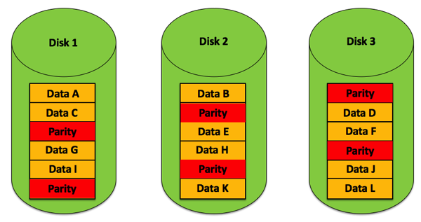
Image source: SQLPassion - How to Calculate RAID 5 Parity Information
In real RAID systems, this XOR operation happens on stripe units—typically 64KB or larger chunks—not individual bytes. A RAID controller continuously performs these calculations across millions of blocks, creating a web of mathematical relationships that can reconstruct any single failed drive from the surviving ones.
The RAID Taxonomy: From Striping to Dual Parity
The original Berkeley paper defined five RAID levels, each representing a different trade-off between capacity, performance, and redundancy.
RAID 0: Pure Striping, Zero Redundancy
RAID 0 splits data into blocks and distributes them across all drives in the array. If you write a 1GB file to a 4-disk RAID 0, each drive stores approximately 250MB. The controller reads and writes to all drives simultaneously, achieving throughput that scales linearly with the number of disks.
The mathematics of RAID 0 reliability is brutal. If each drive has an annual failure rate (AFR) of 1%, a single drive has a 99% chance of surviving the year. But a 4-disk RAID 0 array:
$$P_{survive} = 0.99^4 = 0.9606$$The array has only a 96% survival rate—roughly a 4% annual failure rate. Adding more drives makes failure more likely, not less. RAID 0 trades reliability for speed: maximum performance, minimum safety.
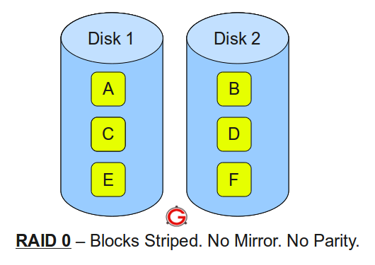
Image source: The Geek Stuff - RAID 0, RAID 1, RAID 5, RAID 10 Explained
RAID 1: Mirroring, Pure Redundancy
RAID 1 takes the opposite approach: every write goes to all drives simultaneously. Each drive contains an identical copy of all data. Read performance improves because the controller can fetch different blocks from different drives in parallel.
The reliability mathematics flips. For a 2-drive mirror, the array fails only if both drives fail. Assuming a 1-day rebuild time, the probability of the second drive failing during rebuild is:
$$P_{second\_fail} = \frac{1}{365} \times 0.01 = 0.000027$$The array’s annual failure rate becomes:
$$P_{array\_fail} = 0.01 \times 0.000027 \times 2 = 0.00000055$$That’s approximately 0.000055%—“six nines” of reliability compared to “two nines” for a single drive. The cost: 50% storage efficiency. You buy 4TB of raw storage but can only store 2TB of data.
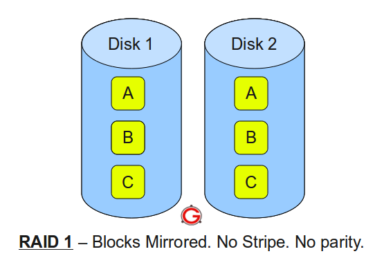
Image source: The Geek Stuff - RAID 0, RAID 1, RAID 5, RAID 10 Explained
RAID 4 and 5: Distributed Parity
RAID 4 introduced the concept of dedicated parity: one disk in the array stores all parity information, while others store data. The XOR relationships allow any single drive to fail and be rebuilt. But RAID 4 has a critical flaw: the parity disk becomes a bottleneck. Every write requires updating parity, meaning the parity disk must participate in every write operation.
RAID 5 solves this by distributing parity across all drives. Instead of one disk handling all parity updates, each drive takes turns storing parity blocks for different stripes. The first stripe might have parity on Drive 1, the second on Drive 2, and so on.
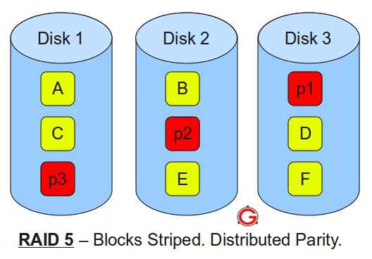
Image source: The Geek Stuff - RAID 0, RAID 1, RAID 5, RAID 10 Explained
The capacity formula for RAID 5 is straightforward. With N drives of capacity C:
$$Usable = (N - 1) \times C$$One drive’s worth of capacity goes to parity. In a 5-drive array with 2TB drives, you get 8TB usable—80% efficiency.
RAID 6: Dual Parity for the Modern Era
As drives grew larger, a problem emerged. Rebuilding a failed 2TB drive takes hours; rebuilding a 20TB drive takes days. During rebuild, every remaining drive must be read completely. The probability of encountering an unrecoverable read error (URE) during this massive read operation became uncomfortably high.
RAID 6 addresses this with double parity. Two independent parity blocks per stripe allow the array to survive any two concurrent drive failures. The parity uses more complex mathematics—often Reed-Solomon coding or specialized XOR variants—but the principle remains: redundancy calculated from data, stored separately, enabling reconstruction.

Image source: Backblaze - NAS RAID Levels Explained
The capacity cost increases: with N drives, usable capacity is (N-2) × C. A 6-drive array with 2TB drives yields 8TB usable—67% efficiency.
RAID 10: The Stripe of Mirrors
RAID 10 combines mirroring and striping in a specific order: first mirror, then stripe. You create pairs of mirrored drives, then stripe data across these mirror pairs. The result combines RAID 0’s performance with RAID 1’s redundancy.
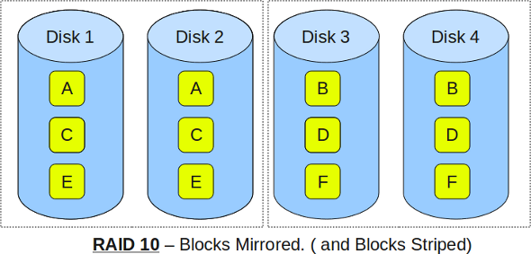
Image source: The Geek Stuff - RAID 0, RAID 1, RAID 5, RAID 10 Explained
A 4-drive RAID 10 consists of two mirror pairs. The array can survive one drive failure per mirror pair—potentially two total failures, as long as they’re in different pairs. If both drives in a single mirror pair fail, all data is lost.
The capacity is always 50% of raw storage, regardless of array size. But the performance is exceptional: full stripe speed for reads and writes, with the redundancy of mirroring.
The Write Penalty: When Redundancy Costs Performance
Parity-based RAID (levels 4, 5, and 6) introduces what storage engineers call the “write penalty.” Understanding this penalty reveals the hidden cost of parity redundancy.
When you write a new block to a RAID 0 array, the controller simply writes the data to the appropriate drive—one operation. But when you modify an existing block in a RAID 5 array, the controller must:
- Read the old data block
- Read the old parity block
- XOR old data with new data
- XOR the result with old parity to get new parity
- Write the new data block
- Write the new parity block
That’s four disk operations for every one logical write—a write penalty of 4. The formula for recalculating parity without reading all data:
$$NewParity = OldData \oplus NewData \oplus OldParity$$This works because XOR is associative and commutative:
$$OldData \oplus OldParity = ParityWithoutOldData$$$$ParityWithoutOldData \oplus NewData = NewParity$$RAID 6 has an even larger write penalty—typically 6 operations per write—because two parity blocks must be updated using more complex calculations involving Galois Field arithmetic.
| RAID Level | Write Penalty | Capacity Efficiency |
|---|---|---|
| RAID 0 | 1 | 100% |
| RAID 1 | 2 | 50% |
| RAID 5 | 4 | (N-1)/N |
| RAID 6 | 6 | (N-2)/N |
| RAID 10 | 2 | 50% |
This explains why RAID 10 often outperforms RAID 5/6 for write-heavy workloads despite its lower capacity efficiency. The trade-off is fundamental: parity RAID trades write performance for capacity efficiency.
The Rebuild Nightmare: When Redundancy Meets Reality
The mathematics of RAID rebuilds reveals a growing problem as drive capacities increase.
Consider a 10-drive RAID 5 array with 10TB drives. When one drive fails, the controller must read 90TB of data from the remaining drives to reconstruct the failed one. At 150 MB/s sustained read speed, this takes:
$$RebuildTime = \frac{90 \times 10^{12}}{150 \times 10^6} \approx 600,000 \text{ seconds} \approx 7 \text{ days}$$During this week-long rebuild, every remaining drive operates under stress. More critically, the probability of encountering an unrecoverable read error increases with the amount of data read.
Consumer-grade drives typically specify a URE rate of 1 in $10^{14}$ bits read—roughly one error per 12.5 TB. Enterprise drives offer $10^{15}$ or better. But when reading 90TB during rebuild, even enterprise drives face meaningful error probability:
$$P_{URE} = 1 - (1 - \frac{1}{10^{15}})^{90 \times 8 \times 10^{12}} \approx 0.5\%$$If a URE occurs during RAID 5 rebuild, the rebuild fails. That single sector—and potentially the entire array—becomes unrecoverable.

Image source: SQLPassion - How to Calculate RAID 5 Parity Information
This is why storage engineers now recommend RAID 6 or RAID 10 for arrays with large drives. RAID 6 can survive a URE during rebuild because it has two parity blocks—losing one sector during rebuild doesn’t lose the array. RAID 10 rebuilds are faster (only need to copy from the mirror, not reconstruct) and don’t require reading all remaining drives.
The Hardware-Software Divide
RAID can be implemented in hardware or software, and the distinction matters.
Hardware RAID uses a dedicated controller card with its own processor, cache memory, and often battery-backed write cache. The controller handles all parity calculations and drive management, offloading the main CPU. The battery backup (or flash-based protection) ensures that writes in progress during power loss can complete when power returns.
Software RAID runs entirely in the operating system kernel. Linux’s mdadm, Windows Storage Spaces, and ZFS all implement RAID in software. Modern CPUs are fast enough that parity calculation overhead is minimal for most workloads.
The trade-offs:
Hardware RAID advantages:
- Dedicated cache with power-loss protection
- Boot-time independence (array is visible to BIOS/UEFI)
- Consistent performance regardless of host CPU load
Software RAID advantages:
- No vendor lock-in (arrays work on any compatible OS)
- Often lower cost (no dedicated hardware)
- Integration with advanced features (ZFS snapshots, compression)
- Portable between systems
For enterprise deployments, hybrid approaches have emerged. “RAID on CPU” implementations use the host CPU for calculations but include a cache module with battery protection. Software-defined storage systems like Ceph distribute RAID-like redundancy across entire clusters rather than single servers.
SSDs Change the Equation
Solid-state drives have transformed RAID considerations. SSDs have no moving parts, eliminating mechanical failure modes. But they introduce new concerns:
Wear leveling and write amplification: SSDs wear out after a finite number of write cycles. RAID’s write penalty accelerates this wear. A RAID 5 array can reduce SSD lifespan by 4× compared to single-drive usage.
TRIM support: TRIM commands tell SSDs which blocks are no longer in use, allowing internal garbage collection. Many hardware RAID controllers don’t pass TRIM through to drives, degrading performance over time.
Performance characteristics: SSDs have different performance profiles than HDDs. They handle random I/O far better, making some RAID design decisions (stripe size optimization) less critical. But they also have different failure modes—often failing into read-only mode rather than disappearing entirely.
For SSD arrays, RAID 10 is often preferred over RAID 5/6. The lower write penalty means less write amplification, extending drive lifespan. The faster rebuild times reduce exposure window during degraded operation.
ZFS and the Evolution Beyond Traditional RAID
Traditional RAID has a fundamental weakness: it trusts that drives report errors honestly. If a drive silently corrupts data but reports success, RAID dutifully replicates or parity-protects that corruption.
ZFS (and similar copy-on-write filesystems) addresses this by integrating RAID-like redundancy with end-to-end checksumming. Every block has a cryptographic checksum, and the filesystem verifies data on every read. When corruption is detected, ZFS can repair it from redundancy if available.
ZFS RAID-Z (analogous to RAID 5) avoids the “write hole” vulnerability of traditional RAID. In conventional RAID 5, if power fails after new data is written but before parity is updated, the stripe becomes inconsistent. RAID-Z’s copy-on-write design writes entire stripes atomically—either the whole stripe writes or none of it does.
For modern storage systems, ZFS or similar integrated approaches often provide better data integrity than traditional RAID alone. The combination of redundancy and verification catches errors that RAID’s XOR mathematics cannot.
Why RAID Is Not a Backup
This point cannot be emphasized enough: RAID provides redundancy, not backup.
The distinction is critical. RAID protects against drive failure—a hardware fault that makes data inaccessible. RAID does not protect against:
- Accidental deletion: If you delete a file, RAID immediately deletes it from all drives or parity sets
- Corruption: If an application corrupts a file, RAID faithfully preserves the corruption
- Ransomware: If malware encrypts your files, RAID ensures all copies are encrypted
- Theft or disaster: If the server is stolen or destroyed, RAID goes with it
- Controller failure: Hardware RAID arrays may not be readable without a compatible controller
Backup implies a separate copy, stored separately, with version history. RAID 1 mirroring gives you two identical copies of your data, but both are live, both are immediately affected by any change, and both are in the same physical location.
A proper backup strategy includes:
- 3-2-1 rule: Three copies of data, on two different media types, with one copy off-site
- Version history: Ability to restore previous versions, not just current state
- Separation: Backup systems isolated from production systems
- Testing: Regular verification that backups can be restored
RAID is a availability feature—it keeps your system running when hardware fails. Backup is a recovery feature—it gets your data back when something goes wrong. They serve different purposes and complement each other.
The Modern RAID Decision
Choosing a RAID level in 2025 involves more factors than the original Berkeley researchers could have imagined:
Drive capacity matters enormously. With 20TB+ drives common, rebuild times stretch to days. RAID 5 is increasingly risky for large drives; RAID 6 or RAID 10 are safer choices.
Workload characteristics drive the decision. Write-heavy databases prefer RAID 10. Read-heavy file servers can use RAID 5/6 effectively. Archival storage might choose RAID 6 for maximum capacity efficiency.
Cost sensitivity shapes choices. RAID 10’s 50% efficiency means buying twice the raw storage you need. For budget-constrained deployments, RAID 6’s (N-2)/N efficiency is attractive.
Data criticality determines redundancy level. Non-critical data might tolerate RAID 5’s single-drive fault tolerance. Mission-critical systems need RAID 6 or RAID 10’s multi-drive tolerance.
Future growth must be considered. Some RAID implementations allow online capacity expansion. Others require backup and rebuild to add drives.
The mathematics of RAID remain constant: XOR parity creates relationships that enable reconstruction. But the practical application has evolved dramatically since 1987. Larger drives, faster processors, SSDs, and integrated filesystems have changed the calculus. What hasn’t changed is the fundamental insight: by combining multiple failure-prone components with careful redundancy, we can build systems more reliable than any individual component.
References
-
Patterson, D. A., Gibson, G. A., & Katz, R. H. (1988). “A Case for Redundant Arrays of Inexpensive Disks (RAID).” ACM SIGMOD Record, 17(3), 109-116.
-
Chen, P. M., Lee, E. K., Gibson, G. A., Katz, R. H., & Patterson, D. A. (1994). “RAID: High-Performance, Reliable Secondary Storage.” ACM Computing Surveys, 26(2), 145-185.
-
SQLPassion. (2017). “How to Calculate RAID 5 Parity Information.” https://www.sqlpassion.at/archive/2017/05/08/how-to-calculate-raid-5-parity-information/
-
Backblaze. (2025). “NAS RAID Levels Explained: Which Level Is Right For You.” https://www.backblaze.com/blog/nas-raid-levels-explained-choosing-the-right-level-to-protect-your-nas-data/
-
The Geek Stuff. (2010). “RAID 0, RAID 1, RAID 5, RAID 10 Explained with Diagrams.” https://www.thegeekstuff.com/2010/08/raid-levels-tutorial/
-
Boolean World. (2024). “RAID Levels 0, 1, 4, 5, 6, 10 Explained.” https://www.booleanworld.com/raid-levels-explained/
-
Wikipedia. “Standard RAID Levels.” https://en.wikipedia.org/wiki/Standard_RAID_levels
-
Plank, J. S. (2008). “The RAID-6 Liberation Codes.” USENIX FAST ‘08. https://www.usenix.org/event/fast08/tech/full_papers/plank/plank.pdf
-
Klennet Software. (2019). “ZFS RAIDZ vs. Traditional RAID.” https://www.klennet.com/notes/2019-07-04-raid5-vs-raidz.aspx
-
StarWind Software. (2024). “Software RAID vs. Hardware RAID.” https://www.starwindsoftware.com/blog/software-raid-vs-hardware-raid-what-is-the-difference/
-
Arcserve. (2024). “Understanding RAID Performance at Various Levels.” https://www.arcserve.com/blog/understanding-raid-performance-various-levels
-
MassiveGrid. (2025). “Understanding RAID Write Penalties: RAID 0, 1, 5, and 6 Explained.” https://www.massivegrid.com/blog/understanding-raid-write-penalties-raid-0-1-5-and-6-explained/
-
TechTarget. (2025). “RAID 5 vs. RAID 6: Capacity, Performance, Durability.” https://www.techtarget.com/searchdatabackup/tip/RAID-5-vs-RAID-6-Capacity-performance-durability
-
Xinnor. (2023). “RAID in the Era of SSDs.” https://xinnor.io/blog/a-guide-to-raid-pt-3-raid-in-the-era-of-ssds/
-
ServerFault. (2009). “Why is RAID not a backup?” https://serverfault.com/questions/2888/why-is-raid-not-a-backup
-
Computer History Museum. “1988: U.C. Berkeley Paper Catalyzes Interest in RAID.” https://www.computerhistory.org/storageengine/u-c-berkeley-paper-catalyses-interest-in-raid/