When you type a query and hit enter, results appear in under half a second. Behind that instant response lies an engineering marvel: a system that must search through hundreds of billions of documents, score each one for relevance, and return the best matches—all before you can blink.
The numbers are staggering. Google’s index contains approximately 400 billion documents according to testimony from their VP of Search during the 2023 antitrust trial. The index itself exceeds 100 million gigabytes. Yet the median response time for a search query remains under 200 milliseconds.
How does this work? The answer involves three fundamental stages: building an index that makes searching possible, ranking documents to surface the most relevant results, and distributing the entire system across thousands of machines. Each stage contains decades of accumulated engineering wisdom.
The Inverted Index: The Heart of Search
A search engine cannot scan every document for every query—that would take hours. Instead, it builds a data structure that inverts the relationship between documents and words.
In a traditional (forward) index, you store documents and the words they contain. Document 1 contains words A, B, C. Document 2 contains words B, D, E. To find documents containing word B, you would need to scan every document.
An inverted index flips this structure. Each unique word (term) becomes a key that points to a list of documents containing that term. This list is called a posting list. When you search for “giraffe,” the engine doesn’t scan documents—it looks up “giraffe” in the term dictionary and retrieves the posting list instantly.
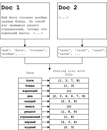
Image source: Summa Blog - How Search Engines Work
The posting list doesn’t just store document IDs. Modern implementations include term frequency (how many times the word appears), position information (where in the document), and various metadata for scoring. A posting list entry might look like: (docID: 48291, tf: 5, positions: [12, 45, 89, 203, 567]).
The Compression Challenge
Posting lists grow enormous. The word “the” appears in nearly every English document—a posting list for it could contain billions of entries. Storing these lists efficiently becomes critical.
The key insight is that document IDs in a posting list are always sorted in ascending order. Instead of storing [1, 5, 7, 12, 18, 25], we can store the gaps: [1, 4, 2, 5, 6, 7]. These smaller numbers compress better using variable-length encoding schemes like varint, which uses fewer bytes for smaller numbers.

Image source: Stanford NLP Group - Introduction to Information Retrieval
Skip pointers add another optimization. By embedding occasional “jump” references within posting lists, search engines can skip over entire sections when merging lists for multi-term queries. The heuristic of using $\sqrt{P}$ evenly-spaced skip pointers for a list of length $P$ has proven effective in practice.
From Matches to Rankings: The Relevance Problem
Finding documents that contain your search terms is only half the battle. A query for “apple” might match millions of documents about fruit, technology, and music. How does the engine decide which results belong on the first page?
BM25: The Workhorse Ranking Function
Most search engines use BM25 (Best Matching 25) as their primary relevance scoring algorithm. Developed in the 1980s and 1990s by researchers at City University London, BM25 remains the default ranking function in systems like Elasticsearch and Apache Lucene.
The BM25 formula for scoring a document $d$ against a query $q$ is:
$$score(q, d) = \sum_{t \in q} \frac{tf(t, d) \cdot (k_1 + 1)}{tf(t, d) + k_1 \cdot (1 - b + b \cdot \frac{dl(d)}{avgdl})} \cdot \log\frac{N - df(t) + 0.5}{df(t) + 0.5}$$Let’s break this down:
- $tf(t, d)$: Term frequency—how many times term $t$ appears in document $d$
- $df(t)$: Document frequency—how many documents contain term $t$
- $N$: Total number of documents in the collection
- $dl(d)$: Length of document $d$
- $avgdl$: Average document length across the collection
- $k_1$: Controls term frequency saturation (typically 1.2)
- $b$: Controls document length normalization (typically 0.75)
The brilliance of BM25 lies in two design decisions. First, the saturation function $\frac{tf \cdot (k_1 + 1)}{tf + k_1}$ prevents a document from gaming the system by repeating a word thousands of times. After a certain point, additional occurrences provide diminishing returns. Second, document length normalization penalizes excessively long documents that might mention a term by chance rather than as a core topic.

Image source: Summa Blog - How Search Engines Work
The graph above shows how the saturation function behaves with different $k_1$ values. Higher $k_1$ means term frequency continues to matter more at higher counts.
PageRank: The Authority Signal
BM25 scores document-query similarity. But some documents are inherently more authoritative than others. This is where PageRank, the algorithm that made Google famous, comes in.
Invented by Larry Page and Sergey Brin at Stanford in 1996, PageRank models web behavior as a “random surfer.” Imagine someone randomly clicking links across the web. Pages that receive many links from other important pages will be visited more frequently.
The PageRank formula:
$$PR(A) = (1 - d) + d \cdot \sum_{T_i \rightarrow A} \frac{PR(T_i)}{C(T_i)}$$- $PR(A)$: PageRank of page A
- $d$: Damping factor (typically 0.85), representing the probability the surfer continues clicking
- $T_i$: Pages linking to A
- $C(T_i)$: Number of outbound links from page $T_i$
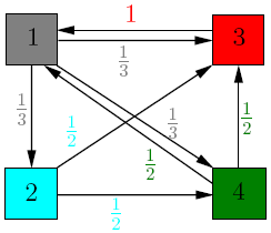
Image source: Cornell University - Mathematics of Google Search
The intuition is democratic: each page “votes” for the pages it links to by distributing its PageRank equally among its outbound links. A link from a high-PageRank page (like Wikipedia) carries more weight than a link from an obscure blog.
Modern search engines combine hundreds of signals—BM25 for text relevance, PageRank for authority, freshness for time-sensitive queries, personalization based on location and history. The exact weighting remains a closely guarded secret, but the principle is clear: relevance is multi-dimensional.
Query Processing: From Keywords to Results
When a query arrives, it undergoes a pipeline of transformations before the engine returns results.
Query Understanding
First, the query must be parsed and understood. This involves:
- Tokenization: Breaking the query into individual terms
- Normalization: Lowercasing, removing diacritics
- Stemming/Lemmatization: Reducing words to root forms (“running” → “run”)
- Stop word handling: Deciding whether to include common words like “the”
- Spelling correction: Identifying and fixing typos
- Query expansion: Adding synonyms and related terms
For the query “best restaraunts NYC,” the engine might expand it to include “restaurants New York City” and correct “restaraunts” to “restaurants.”
Posting List Intersection
For multi-term queries, the engine must find documents containing all (or some) of the terms. With posting lists sorted by document ID, this becomes a merge operation similar to the merge step in merge sort.
For an AND query, we walk through posting lists simultaneously, advancing pointers and collecting matches. For an OR query, we collect documents from all lists, summing their scores.

Image source: Summa Blog - How Search Engines Work
The WAND (Weak AND) optimization dramatically speeds up this process. Instead of scoring every document, WAND maintains a threshold based on the current top-K results and skips documents that cannot possibly make the cut. The Block-max WAND extension stores upper bounds for each block of the posting list, enabling even more aggressive skipping.
The Top-K Heap
Users rarely look beyond the first page of results. Search engines exploit this by using a min-heap of size K (typically 10-100) rather than sorting all matching documents. As each document is scored, it enters the heap only if its score exceeds the current minimum. This reduces memory usage and avoids sorting millions of scores.
Distributed Architecture: Scaling to Billions
A single machine cannot store or search 400 billion documents. Search engines distribute the index across thousands of servers using sharding.
Index Sharding
Documents are assigned to shards based on their ID (often using consistent hashing). Each shard contains a complete inverted index for its subset of documents. When a query arrives, it’s broadcast to all shards in parallel. Each shard returns its top results, and a coordinator merges these into the final result set.
This architecture provides both scalability and fault tolerance. If a shard fails, results may be slightly incomplete but the system stays operational. Capacity can be added by creating new shards.
The Crawler: Keeping the Index Fresh
Web content changes constantly. Pages are created, modified, and deleted. A web crawler must continuously discover and re-fetch content to keep the index current.
Crawling presents unique challenges. A crawler must respect robots.txt directives, avoid overwhelming servers (politeness), prioritize high-value pages (scheduling), and handle the internet’s scale. Google’s crawler, Googlebot, runs across thousands of machines using a distributed architecture managed by systems like Borg (Google’s internal cluster manager).
The freshness problem has no perfect solution. News sites need re-crawling every minute; academic papers might change once per decade. Sophisticated scheduling algorithms estimate change probability based on historical update patterns and page importance.
Storage: Immutable Segments
Modern search engines like Apache Lucene (which powers Elasticsearch and Solr) use an immutable, append-only storage model. When documents are added or updated, new index segments are created rather than modifying existing ones.
This approach has several advantages. Immutable segments are cache-friendly, can be memory-mapped directly, and enable efficient snapshots. When too many small segments accumulate, they’re merged in the background—a process that can be computationally expensive but doesn’t block queries.
The Evolution Continues
The inverted index and BM25 remain the foundation of search, but the field evolves constantly. Neural ranking models using transformer architectures like BERT now complement traditional algorithms, capturing semantic meaning that keyword matching misses. Vector search represents documents as dense embeddings in high-dimensional space, enabling similarity-based retrieval.
Hybrid search systems combine these approaches: BM25 for precise keyword matching, vector search for semantic similarity, with results fused using reciprocal rank fusion or learned scoring. Google’s integration of BERT into search in 2019 marked a shift toward neural understanding, though the fundamental infrastructure of inverted indexes remains.
The next time you search and see results in milliseconds, remember: you’re benefiting from 30 years of accumulated engineering—a system that has solved the impossible problem of finding exactly what you need among billions of possibilities, instantly.
References
-
Brin, S., & Page, L. (1998). The Anatomy of a Large-Scale Hypertextual Web Search Engine. Computer Networks and ISDN Systems, 30(1-7), 107-117. http://infolab.stanford.edu/~backrub/google.html
-
Robertson, S., & Zaragoza, H. (2009). The Probabilistic Relevance Framework: BM25 and Beyond. Foundations and Trends in Information Retrieval, 3(4), 333-389.
-
Manning, C. D., Raghavan, P., & Schütze, H. (2008). Introduction to Information Retrieval. Cambridge University Press. https://nlp.stanford.edu/IR-book/
-
Cornell University Department of Mathematics. (2009). Lecture #3: PageRank Algorithm - The Mathematics of Google Search. https://pi.math.cornell.edu/~mec/Winter2009/RalucaRemus/Lecture3/lecture3.html
-
Broder, A. Z., Carmel, D., Herscovici, M., Soffer, A., & Zien, J. (2003). Efficient Query Evaluation using a Two-Level Retrieval Process. Proceedings of the Twelfth International Conference on Information and Knowledge Management, 426-434.
-
Ding, S., & Suel, T. (2011). Faster Top-k Document Retrieval using Block-Max Indexes. Proceedings of the 34th International ACM SIGIR Conference on Research and Development in Information Retrieval, 993-1002.
-
Google. How Search Works. https://www.google.com/intl/en_us/search/howsearchworks/
-
Zyppy. Google’s Index Size Revealed: 400 Billion Docs. https://zyppy.com/seo/google-index-size/
-
Summa. How Search Engines Work: Base Search and Inverted Index. https://izihawa.github.io/summa/blog/how-search-engines-work/
-
Elastic. Practical BM25 - Part 2: The BM25 Algorithm and its Variables. https://www.elastic.co/blog/practical-bm25-part-2-the-bm25-algorithm-and-its-variables