In 1952, a graduate student at MIT named David Huffman faced a choice: write a term paper or take a final exam. His professor, Robert Fano, had assigned a paper on finding the most efficient binary code—a problem that had stumped both Fano and Claude Shannon, the father of information theory. Huffman, unable to prove any existing codes were optimal, was about to give up and start studying for the final. Then, in a flash of insight, he thought of building the code tree from the bottom up rather than the top down. The result was optimal, elegant, and would become one of the most widely used algorithms in computing history.
Huffman coding is just one piece of the compression puzzle. The ZIP file on your computer, the PNG images on websites, the HTTP responses from servers—all rely on a combination of mathematical insights that span decades. Understanding how these algorithms work reveals something fundamental about information itself: what it means to be redundant, and what it means to be truly random.
Shannon’s Impossible Compression
Before any compression algorithm can work, there must be something to compress. In 1948, Claude Shannon published “A Mathematical Theory of Communication,” founding the field of information theory. Among his key insights was the concept of entropy—a measure of how much information a message contains.
Shannon entropy, denoted $H(X)$, is calculated as:
$$H(X) = -\sum_{i=1}^{n} p_i \log_2 p_i$$Where $p_i$ is the probability of the $i$-th symbol appearing. The result tells you the minimum average number of bits needed to encode each symbol. If a message has high entropy—meaning each symbol is equally likely and unpredictable—Shannon proved that no compression algorithm can make it smaller without losing information.
This theorem established a fundamental limit. If you have 256 equally likely symbols, each requires exactly 8 bits to encode. No clever algorithm can change this. Compression only works when some symbols are more likely than others, creating what Shannon called “redundancy.”
Consider English text. The letter ’e’ appears about 12.7% of the time, while ‘z’ appears only 0.07% of the time. This non-uniform distribution means English text carries less information per character than a random sequence—and therefore can be compressed. Shannon estimated English text has an entropy of about 2.1 bits per character, far below the 8 bits used in standard ASCII encoding.
Huffman’s Optimal Trees
Huffman’s algorithm exploits this non-uniformity by assigning shorter codes to more frequent symbols. The algorithm is remarkably simple:
- Create a leaf node for each symbol, weighted by its frequency
- Repeatedly combine the two nodes with lowest weights into a new internal node
- The weight of the new node is the sum of its children’s weights
- Continue until only one node remains—the root of the tree
Reading codes from the tree is straightforward: assign ‘0’ for left branches and ‘1’ for right branches. The path from root to leaf gives the code for that symbol.
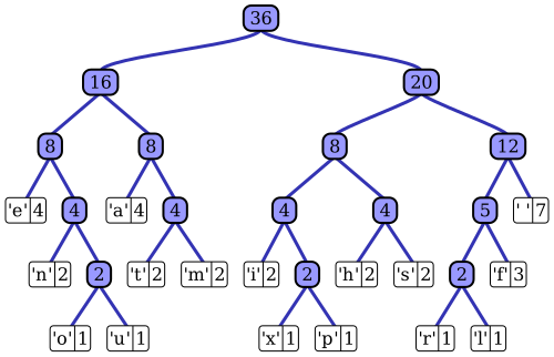
Image source: Wikipedia - Huffman Coding
The table above shows a complete Huffman code for a sample text. Notice how common characters like ‘space’ (7 occurrences) get short 3-bit codes, while rare characters like ‘x’ (1 occurrence) get longer 5-bit codes. The beauty of Huffman coding is that no code is a prefix of any other—you can always tell when one symbol ends and the next begins.
flowchart TD
    A[Symbol Frequencies] --> B[Create Leaf Nodes]
    B --> C[Sort by Frequency]
    C --> D{More than 1 node?}
    D -->|Yes| E[Combine 2 lowest]
    E --> F[Add weights]
    F --> C
    D -->|No| G[Build Complete Tree]
    G --> H[Assign Codes: 0=left, 1=right]
    H --> I[Optimal Prefix-Free Code]
The diagram above shows the Huffman tree construction process, from initial frequencies to the final optimal code.
Huffman proved his algorithm produces the optimal prefix-free code for any given probability distribution. The expected code length approaches Shannon entropy arbitrarily closely as the number of symbols increases. For the example in the table, the weighted average code length is 2.25 bits per symbol—only slightly above the calculated entropy of 2.205 bits.
The Sliding Window Breakthrough
But Huffman coding alone has a limitation: it only exploits symbol frequency, not patterns across multiple symbols. The phrase “the the the the” would compress poorly with pure Huffman coding, even though it’s clearly redundant.
In 1977, Abraham Lempel and Jacob Ziv published a radically different approach. Rather than assigning codes based on frequency, LZ77 maintains a “sliding window” of recently seen data. When the algorithm encounters a sequence that appeared before, it replaces it with a back-reference: a pair of numbers indicating “go back X bytes and copy Y bytes.”
The sliding window typically holds 32KB of data. For each position, the encoder searches backwards through the window for the longest matching sequence. If a match is found, it outputs a length-distance pair; otherwise, it outputs the literal byte.
flowchart LR
    subgraph SlidingWindow["Sliding Window (32KB)"]
        SearchBuffer["Search Buffer<br/>(Previously seen)"]
        Lookahead["Lookahead Buffer<br/>(To be encoded)"]
    end

    Input["Input Stream"] --> SlidingWindow
    SearchBuffer --> Match{"Find match?"}
    Match -->|Yes| Output1["Output: (distance, length)"]
    Match -->|No| Output2["Output: literal byte"]
    Output1 --> Compressed["Compressed Stream"]
    Output2 --> Compressed
The diagram above illustrates the LZ77 sliding window concept: previously seen data forms a search buffer, and matches are replaced with back-references.
Consider compressing the string “ABRACADABRA”. After processing “ABRACAD”, the window contains these characters. When the algorithm reaches the second “ABRA”, it finds a match 7 bytes back with length 4. Instead of outputting four bytes, it outputs a single back-reference. For repetitive text, this can achieve dramatic compression.
A clever aspect of LZ77 is that the length can exceed the distance. If you want to encode “AAAAAAAA” (8 A’s) and there’s a single ‘A’ one byte back, the encoder can output a reference to copy 8 bytes starting 1 byte back. The decoder copies the first ‘A’, which then becomes available for copying the next ‘A’, and so on—like a snake eating its own tail.
DEFLATE: The Marriage of Two Ideas
In 1990, Phil Katz combined LZ77 and Huffman coding into a single algorithm called DEFLATE. This algorithm powers ZIP files, gzip compression, PNG images, and the HTTP compression used by virtually every web server.
DEFLATE works in two stages:
- LZ77 Stage: Find repeated sequences and replace them with back-references (length-distance pairs) or literals
- Huffman Stage: Apply Huffman coding to the literals, lengths, and distances from stage 1
The Huffman stage is where DEFLATE gets clever. It doesn’t use a single Huffman tree—it uses two: one for literals and lengths, another for distances. These trees can be dynamic (built for each block of data) or static (predefined by the specification).
flowchart LR
    A[Raw Data] --> B[LZ77 Encoding]
    B --> C[Literals + Length/Distance Pairs]
    C --> D[Huffman Coding]
    D --> E[Compressed Bitstream]

    F[Sliding Window<br/>32KB] --> B
    G[Huffman Trees<br/>Dynamic or Static] --> D
The flowchart above shows how DEFLATE combines LZ77 and Huffman coding to produce compressed output.
A DEFLATE stream consists of blocks, each with a 3-bit header. The header indicates whether the block is uncompressed (useful for incompressible data), uses static Huffman trees, or uses dynamic Huffman trees. Most compressible data ends up in dynamic blocks, where the Huffman trees are optimized for each block’s specific symbol distribution.
PNG: When Filtering Matters More Than Compression
PNG images demonstrate another crucial insight: what you compress matters as much as how you compress it. PNG doesn’t just apply DEFLATE to raw pixel data—it first applies filtering to make the data more compressible.
PNG supports five filter types for each row of pixels:
- None: No filtering (raw data)
- Sub: Subtract the pixel to the left
- Up: Subtract the pixel above
- Average: Subtract the average of left and above pixels
- Paeth: Use a predictor based on three neighboring pixels
The Paeth filter, invented by Alan Paeth, is particularly clever. It calculates a simple linear predictor from the left, above, and upper-left pixels, then chooses the closest predictor among them. For photographs with gradual color changes, this filtering creates long runs of small numbers and zeros—exactly what LZ77 and Huffman coding compress best.
A typical photograph might compress to 40-60% of its original size with PNG. But the same image stored as a screenshot (with large solid-color areas) might compress to 10% or less. The difference isn’t the compression algorithm—it’s the filtering that creates exploitable redundancy.
The Speed-Ratio Trade-off
Modern compression libraries expose a compression level parameter, typically 1-9. Higher levels search harder for matches and build better Huffman trees, at the cost of compression time. Decompression speed remains nearly constant regardless of the level used during compression.
This asymmetry exists because compression requires searching for patterns, while decompression only follows instructions. A decompressor reads length-distance pairs and copies data—no searching required. This makes compression naturally slower than decompression, typically by 3-10x depending on the algorithm and level.
The benchmark data tells a clear story:
| Algorithm | Compression Ratio | Compression Speed | Decompression Speed |
|---|---|---|---|
| LZ4 | ~2.0x | 500+ MB/s | 1000+ MB/s |
| Zstd (level 3) | ~2.8x | 300+ MB/s | 800+ MB/s |
| DEFLATE (level 6) | ~2.5x | 50 MB/s | 150 MB/s |
| Brotli (level 9) | ~3.2x | 10 MB/s | 150 MB/s |
LZ4, developed by Yann Collet, sacrifices compression ratio for blazing speed. It’s designed for scenarios where data is compressed once and decompressed many times—exactly the pattern in web servers and databases. Zstd, also by Collet, offers a more balanced approach with excellent compression ratios at reasonable speeds.
Brotli, developed by Google, achieves the best compression ratios by using a large predefined dictionary of common web strings and more sophisticated context modeling. It’s ideal for static assets that can be compressed once and served millions of times.
Why You Can’t Compress Random Data
Shannon’s theorem implies a hard truth: truly random data cannot be compressed. If every symbol is equally likely and independent, the entropy equals the number of bits. No algorithm can make it smaller.
This leads to a simple test for compression scams: if someone claims to compress random data, they’re lying. The proof is straightforward. If a compressor could make any input smaller, you could run it repeatedly on its own output until you reach a single bit. But a single bit can only represent two values, while the original data could represent infinitely many values. Information is conserved.
Kolmogorov complexity formalizes this: the shortest possible description of a string is the length of the shortest program that outputs that string. For random strings, this complexity equals or exceeds the string length itself. Compression works only when the Kolmogorov complexity is lower than the string length—when there’s structure, pattern, redundancy to exploit.
The Limits of Huffman Coding
Huffman coding, despite its elegance, isn’t always optimal. The problem arises when symbol probabilities don’t align with powers of 2. If a symbol has probability 0.4, the ideal code length is $-\log_2(0.4) \approx 1.32$ bits. But Huffman codes must have integer lengths—either 1 bit or 2 bits.
Arithmetic coding solves this by encoding the entire message as a single fractional number. Rather than assigning codes to individual symbols, it maintains an interval that shrinks with each symbol encoded. The final interval can be represented with fractional bits, achieving compression closer to Shannon’s limit.
For most practical purposes, the gap between Huffman and arithmetic coding is small—typically 1-5% in compression ratio. Huffman remains popular because it’s faster, patent-free, and simpler to implement. DEFLATE uses Huffman, not arithmetic coding, for these reasons.
What Compression Reveals About Information
Lossless compression works because real-world data is rarely random. Text has letter frequencies and word patterns. Images have smooth gradients and repeated colors. Programs have repeated code structures. All of this structure represents redundancy—information that can be predicted from context.
The algorithms we’ve explored—Huffman coding, LZ77, DEFLATE—each exploit a different type of redundancy. Huffman exploits non-uniform symbol frequencies. LZ77 exploits repeated sequences. DEFLATE combines both. PNG filtering creates new redundancy by exploiting spatial correlation in images.
When you compress a file, you’re essentially asking: how much of this data is actually new information? The compression ratio tells you the answer. A text file that compresses to 30% of its original size is 70% redundant—it carries only 30% new information per byte. An already-compressed file that doesn’t shrink further carries nearly 100% new information per byte.
This insight has profound implications beyond storage. Compression algorithms have been used to detect plagiarism, identify languages, classify documents, and measure the similarity between strings. If two files compress better together than separately, they share patterns—they’re related in some way.
David Huffman couldn’t have known in 1952 that his term paper would eventually compress billions of files daily. The algorithms have evolved—LZ77 led to LZ78, which led to LZW (used in GIF). DEFLATE led to Deflate64, which led to the modern zstd. But the core insight remains unchanged: information has structure, and structure can be exploited. The rest is mathematics.
References
-
Huffman, D. A. (1952). “A Method for the Construction of Minimum-Redundancy Codes.” Proceedings of the IRE, 40(9), 1098-1101.
-
Ziv, J., & Lempel, A. (1977). “A Universal Algorithm for Sequential Data Compression.” IEEE Transactions on Information Theory, 23(3), 337-343.
-
Ziv, J., & Lempel, A. (1978). “Compression of Individual Sequences via Variable-Rate Coding.” IEEE Transactions on Information Theory, 24(5), 530-536.
-
Shannon, C. E. (1948). “A Mathematical Theory of Communication.” Bell System Technical Journal, 27(3), 379-423.
-
Deutsch, P. (1996). “DEFLATE Compressed Data Format Specification version 1.3.” RFC 1951, Internet Engineering Task Force.
-
Deutsch, P., & Gailly, J. L. (1996). “ZLIB Compressed Data Format Specification version 3.3.” RFC 1950, Internet Engineering Task Force.
-
Boutell, T., et al. (1997). “PNG (Portable Network Graphics) Specification Version 1.0.” RFC 2083, Internet Engineering Task Force.
-
Collet, Y. (2016). “Smaller and faster data compression with Zstandard.” Facebook Engineering Blog.
-
Alakuijala, J., & Szabadka, Z. (2016). “Brotli Compressed Data Format.” RFC 7932, Internet Engineering Task Force.
-
Collet, Y. (2011). “LZ4: Extremely fast compression algorithm.” GitHub Repository.
-
Cover, T. M., & Thomas, J. A. (2006). Elements of Information Theory (2nd ed.). Wiley-Interscience.
-
Salomon, D. (2007). Data Compression: The Complete Reference (4th ed.). Springer.
-
Li, M., & Vitányi, P. (2008). An Introduction to Kolmogorov Complexity and Its Applications (3rd ed.). Springer.
-
Rissanen, J. (1976). “Generalized Kraft Inequality and Arithmetic Coding.” IBM Journal of Research and Development, 20(3), 198-203.
-
Nelson, M. (1991). The Data Compression Book. M&T Books.
-
Witten, I. H., Neal, R. M., & Cleary, J. G. (1987). “Arithmetic Coding for Data Compression.” Communications of the ACM, 30(6), 520-540.