When 0.1 + 0.2 ≠ 0.3: The IEEE 754 Standard That Broke Your Calculations

Type 0.1 + 0.2 into any browser console, Python REPL, or JavaScript runtime. The answer comes back as 0.30000000000000004. This isn’t a bug. It’s not an error in your programming language. It’s the inevitable consequence of a fundamental tension: humans count in base 10, but computers count in base 2.

The IEEE 754 floating-point standard, adopted in 1985, unified how computers represent decimal numbers. Before this standard, different machines handled floating-point arithmetic differently—code that worked on one system could produce completely different results on another. William Kahan, the primary architect of IEEE 754, designed a system that traded perfect precision for predictability. Every programmer would get the same answer, even if that answer wasn’t mathematically exact.

The Binary Representation Problem

The core issue stems from how fractions work in different number bases. In base 10, only fractions with denominators containing prime factors of 2 and 5 can be expressed exactly. This is why 1/3 = 0.333… repeats forever—3 is not a prime factor of 10. But 1/4 = 0.25 terminates cleanly because 4 = 2².

In binary (base 2), the only prime factor is 2 itself. This means only fractions with denominators that are powers of 2 can be represented exactly. The decimal 0.5 equals 1/2, which is 0.1 in binary—perfectly clean. But 0.1 in decimal equals 1/10, and 10 contains the prime factor 5. In binary, 0.1 becomes:

0.0001100110011001100110011001100110011...

This pattern repeats forever. The binary expansion of 0.2 (1/5) is similarly infinite:

0.0011001100110011001100110011001100110...

A 64-bit double-precision floating-point number has only 53 bits for the significand (the fractional part). When the computer stores 0.1, it must truncate this infinite expansion and round to the nearest representable value. The same happens with 0.2. When you add these two approximations together, the rounding errors compound, producing a result that’s slightly different from 0.3.

Inside IEEE 754: The Three-Component Architecture

A floating-point number consists of three parts: sign, exponent, and significand (also called mantissa). The standard defines several formats, but the two most common are:

Single precision (32-bit float):

• 1 bit for sign (0 = positive, 1 = negative)
• 8 bits for exponent (biased by 127)
• 23 bits for significand

Double precision (64-bit float):

• 1 bit for sign
• 11 bits for exponent (biased by 1023)
• 52 bits for significand

The actual value represented is: $(-1)^{sign} \times 1.fraction \times 2^{(exponent - bias)}$

The “1.” before the fraction is implicit—since normalized binary numbers always start with 1, there’s no need to store it explicitly. This gives you one extra bit of precision for free.

Image source: GeeksforGeeks - IEEE Standard 754 Floating Point Numbers

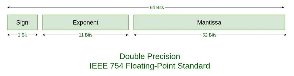
Image source: GeeksforGeeks - IEEE Standard 754 Floating Point Numbers

The exponent uses a biased representation rather than two’s complement. For double precision, the actual exponent is the stored value minus 1023. This makes comparing floating-point numbers as simple as comparing their bit patterns as integers—the ordering is preserved.

Fabien Sanglard offers an intuitive way to visualize this: think of the exponent as a “window” between consecutive powers of two, and the significand as an “offset” within that window. The window [0.5, 1] has 8,388,608 possible offsets (for single precision), giving a granularity of about $1.19 \times 10^{-7}$. But the window [2048, 4096] has the same number of offsets covering a much larger range, so each offset represents a step of about 0.0002—a loss of three decimal places of precision.

The Uneven Distribution of Numbers

Floating-point numbers are not evenly distributed along the number line. They cluster densely near zero and become increasingly sparse as magnitude grows. Between 1.0 and 2.0, there are $2^{52}$ representable doubles (about 4.5 quadrillion values). Between 2.0 and 4.0, the same number of values must cover twice the range, so the gaps double. Between $2^{52}$ and $2^{53}$, the gap between consecutive floating-point numbers is exactly 1—integers in this range can still be represented exactly, but above $2^{53}$, even integers become sparse.

This uneven distribution has practical consequences. Adding a small number to a large number may produce no change at all if the small number is smaller than the gap between representable values near the large number. For single-precision floats, adding 1.0 to 16,777,216.0 produces 16,777,216.0—the 1 is lost entirely because the gap at that magnitude is 2.

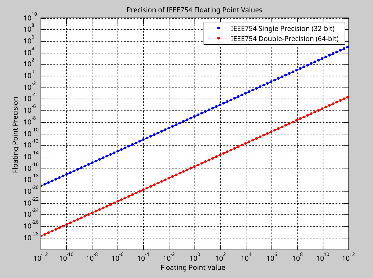
Image source: Wikipedia - IEEE 754

The machine epsilon (ε) defines the upper bound on relative rounding error. For double precision, $\varepsilon = 2^{-52} \approx 2.22 \times 10^{-16}$. This means if you compute $1 + \varepsilon/2$, the result rounds back to exactly 1. The smallest number that, when added to 1, produces a different result is $\varepsilon$ itself.

Real-World Disasters: When Precision Failed

The abstract mathematics of floating-point arithmetic has claimed real lives and destroyed real fortunes.

The Patriot Missile Failure (1991)

On February 25, 1991, during the Gulf War, a U.S. Patriot missile battery in Dhahran, Saudi Arabia, failed to intercept an incoming Iraqi Scud missile. The Scud struck an Army barracks, killing 28 soldiers and injuring approximately 100 others.

The cause was a subtle time-keeping error. The Patriot’s internal clock measured time in tenths of a second, stored as an integer. To convert to seconds, the system multiplied by 1/10. But 1/10 cannot be represented exactly in binary—it’s a repeating fraction. The software used a 24-bit approximation, introducing an error of about $9.5 \times 10^{-8}$ per tenth-second.

This error seems tiny, but the system had been running continuously for about 100 hours. The accumulated error: approximately 0.34 seconds. A Scud missile travels at roughly 1,676 meters per second. In 0.34 seconds, it covers more than 500 meters—enough to move completely outside the “range gate” the Patriot used to track targets. The system was looking in the wrong place.

The Ariane 5 Explosion (1996)

On June 4, 1996, the European Space Agency’s Ariane 5 rocket exploded 37 seconds after liftoff, destroying $500 million in rocket and payload. The cause: code reuse from Ariane 4 that performed an unprotected conversion from a 64-bit floating-point number to a 16-bit signed integer.

The horizontal velocity value, which was safe for Ariane 4’s flight profile, exceeded 32,767—the maximum value storable in a 16-bit signed integer. The conversion overflowed, causing the guidance system to fail. The rocket veered off course and triggered its self-destruct sequence.

Knight Capital (2012)

On August 1, 2012, Knight Capital Group lost $440 million in 45 minutes due to a software deployment error. While not directly caused by floating-point issues, it exemplifies how numerical errors in automated trading systems can cascade catastrophically. A flag used to differentiate between old and new code was left in a “live” state, causing the system to simultaneously execute both old and new trading logic, sending erroneous orders at high speed.

Special Values and Edge Cases

IEEE 754 defines several special values to handle edge cases:

Zero: Both +0 and -0 exist. They compare equal but have different bit patterns. This matters when computing functions like 1/x or log(x) where the sign of zero changes the result.

Infinity: Positive and negative infinity result from operations like 1/0 or overflow. Infinity propagates through most operations: $\infty + x = \infty$ (for finite x), but $\infty - \infty$ produces NaN.

NaN (Not a Number): Results from invalid operations like $0/0$, $\infty - \infty$, or $\sqrt{-1}$. NaN has the unusual property that NaN != NaN evaluates to true. This provides a way to check for invalid results without explicit error handling.

Subnormal numbers: When the exponent field is all zeros, the implicit leading 1 becomes a 0, and the exponent is fixed at -126 (single) or -1022 (double). This allows gradual underflow—numbers smaller than $2^{-126}$ can still be represented, albeit with decreasing precision. Without subnormals, the smallest positive single-precision number would jump directly to zero.

Rounding Modes: Five Ways to Approximate

IEEE 754 defines five rounding modes:

1. Round to nearest, ties to even (default): Rounds to the nearest representable value. If exactly halfway between two values, chooses the one with an even least significant bit. This eliminates statistical bias.

2. Round to nearest, ties away from zero: Halfway cases round away from zero. Rarely used.

3. Round toward +∞: Always rounds up. Useful for interval arithmetic.

4. Round toward -∞: Always rounds down.

5. Round toward zero: Truncates toward zero.

The default “round to nearest, ties to even” explains why 0.1 + 0.2 produces exactly 0.30000000000000004. The true mathematical sum falls between two representable doubles. The one ending in 4 has an even least significant bit in its significand, so that’s the chosen approximation.

Solutions: How to Handle Floating-Point Precision

For Financial Calculations: Use Decimal Types

Never use binary floating-point for money. Most languages provide decimal types that store numbers in base 10:

• Python: decimal.Decimal
• Java: java.math.BigDecimal
• C#: decimal type (128-bit decimal floating-point)
• JavaScript: Use libraries like decimal.js

from decimal import Decimal
result = Decimal('0.1') + Decimal('0.2')  # Exactly 0.3

Decimal types represent 0.1 exactly because they store numbers in base 10, matching human expectations. The trade-off is performance—decimal arithmetic is significantly slower than binary floating-point.

For Comparisons: Use Epsilon Tolerance

Never compare floating-point numbers for exact equality. Instead, check if they’re “close enough”:

def nearly_equal(a, b, epsilon=1e-10):
    return abs(a - b) < epsilon

# Better: relative epsilon for numbers of different magnitudes
def nearly_equal_relative(a, b, rel_tol=1e-9, abs_tol=0.0):
    return abs(a-b) <= max(rel_tol * max(abs(a), abs(b)), abs_tol)

Python 3.5+ provides math.isclose() with both relative and absolute tolerance. The relative tolerance scales with the magnitude of the numbers, handling both small and large values appropriately.

For Accumulation: Kahan Summation

When summing many numbers, rounding errors accumulate. Kahan summation algorithm compensates for the error:

def kahan_sum(numbers):
    total = 0.0
    compensation = 0.0
    for num in numbers:
        y = num - compensation
        t = total + y
        compensation = (t - total) - y
        total = t
    return total

This can reduce accumulated error from $O(n\varepsilon)$ to $O(\varepsilon)$ for summing n numbers.

For Games and Simulations: Fixed-Point Arithmetic

Game engines often use fixed-point arithmetic for deterministic behavior across platforms. Fixed-point numbers have a fixed number of decimal places, stored as integers. A 32-bit fixed-point number with 16 fractional bits can represent values from -32768 to 32767.99998 with uniform precision.

For Machine Learning: Lower Precision Formats

Modern deep learning uses specialized floating-point formats:

• bfloat16: 16-bit format with 8-bit exponent and 7-bit significand. Same exponent range as float32, but reduced precision. Training neural networks tolerates this imprecision well.
• float16: 5-bit exponent, 10-bit significand. Smaller range, more precision than bfloat16.

The reduced precision actually helps prevent overfitting in some cases, acting as implicit regularization.

The Fundamental Trade-off

IEEE 754 embodies a fundamental trade-off: range versus precision. With 64 bits, you can represent numbers from $2.2 \times 10^{-308}$ to $1.8 \times 10^{308}$, but you cannot represent all numbers in between. The standard chooses a logarithmic distribution that maximizes the effective range while maintaining useful precision for most applications.

This isn’t a flaw—it’s a design decision. The alternative would be fixed-point arithmetic with uniform precision but severely limited range, or arbitrary-precision arithmetic with severe performance costs. IEEE 754 hit a sweet spot that has served computing for four decades.

Understanding floating-point arithmetic isn’t about memorizing edge cases. It’s about recognizing that computers operate in a different mathematical universe than humans. When you write 0.1, you’re not asking the computer to store one-tenth. You’re asking it to find the closest approximation among a finite set of representable values. Sometimes that approximation matches your intent. Sometimes it doesn’t.

The bugs aren’t in the computer. They’re in our assumptions.

References

1. IEEE Standard 754-2019 for Floating-Point Arithmetic. IEEE Computer Society, 2019.

2. Goldberg, David. “What Every Computer Scientist Should Know About Floating-Point Arithmetic.” ACM Computing Surveys, March 1991.

3. Skeel, Robert. “Roundoff Error and the Patriot Missile.” SIAM News, 1992.

4. Lions, J.L. “ARIANE 5 Flight 501 Failure.” European Space Agency, 1996.

5. Kahan, William. “IEEE 754: An Interview with William Kahan.” IEEE Computer Society, 1997.

6. General Accounting Office. “Patriot Missile Defense: Software Problem Led to System Failure at Dhahran, Saudi Arabia.” GAO/IMTEC-92-26, 1992.

7. Sanglard, Fabien. “Floating Point Visually Explained.” fabiensanglard.net, 2017.

8. Quinn, Michael J. “Parallel Programming in C with MPI and OpenMP.” McGraw-Hill, 2004.

9. Higham, Nicholas J. “Accuracy and Stability of Numerical Algorithms.” SIAM, 2002.

10. 0.30000000000000004.com - “Floating Point Math”