In 1947, a mathematician at Bell Labs faced a frustrating problem. Richard Hamming was using the Model V relay computer to perform calculations, and every weekend the machine would grind to a halt when it encountered an error. The computer would simply stop, flashing its error lights, and Hamming would have to wait until Monday for the operators to reload his program. One Friday evening, staring at the silent machine, he asked himself a question that would change computing forever: “Why can’t the computer correct its own mistakes?”
That question led to the invention of error-correcting codes—mathematical structures that have become so ubiquitous we forget they exist. Every QR code you scan, every file stored on your SSD, every satellite transmission from Voyager carries error correction baked into its structure. Without these codes, digital communication as we know it would be impossible.
The Mathematics of Distance
Hamming’s insight was that not all binary strings are created equal. Consider the strings 0000 and 0001—they differ by only one bit. But 0000 and 1111 differ by four bits. Hamming realized this difference could be exploited for error detection.
The Hamming distance between two strings is simply the number of positions where they differ. This seemingly simple concept has profound implications. If you transmit the string 0000 and a single bit flips due to noise, you might receive 0001. But if all valid codewords differ by at least two bits, you can detect that an error occurred—the received string won’t match any valid codeword.
The key insight is that with more distance between codewords, you can do more than detect errors—you can correct them. If valid codewords differ by at least three bits, a single-bit error will produce a string that’s closer to the original codeword than to any other. The mathematics:
$$t = \lfloor \frac{d_{min} - 1}{2} \rfloor$$Where $t$ is the number of correctable errors and $d_{min}$ is the minimum Hamming distance between any two codewords. A distance of 3 allows correction of 1 error. A distance of 7 allows correction of 3 errors.
Parity: The Simplest Detection
Before Hamming’s codes, the primary method of error detection was parity—a single bit added to ensure the total number of 1s is even (or odd). If you’re transmitting 7 bits of data and add an 8th parity bit, you can detect any single-bit error.
But parity can’t correct errors. It can only tell you something went wrong. In Hamming’s weekend frustrations, parity was exactly what the Model V computer used—it would detect an error and halt. What Hamming wanted was a code that could both detect and correct.
The problem with single parity is its distance. If you transmit 0000 with even parity (00000), and a bit flips, you get 00100 or 01000 or similar. These are all invalid—but you can’t tell which bit flipped. The minimum distance is only 2, allowing detection but not correction.
Hamming Codes: The Breakthrough
Hamming’s solution was elegant: use multiple parity bits, each checking different overlapping subsets of the data bits. For a Hamming(7,4) code, you transmit 4 data bits plus 3 parity bits, for a total of 7 bits.
The trick lies in which bits each parity bit checks. Position the bits at positions 1, 2, 4, 8, … (powers of 2). Each parity bit checks all positions where that power of 2 appears in the binary representation of the position number.
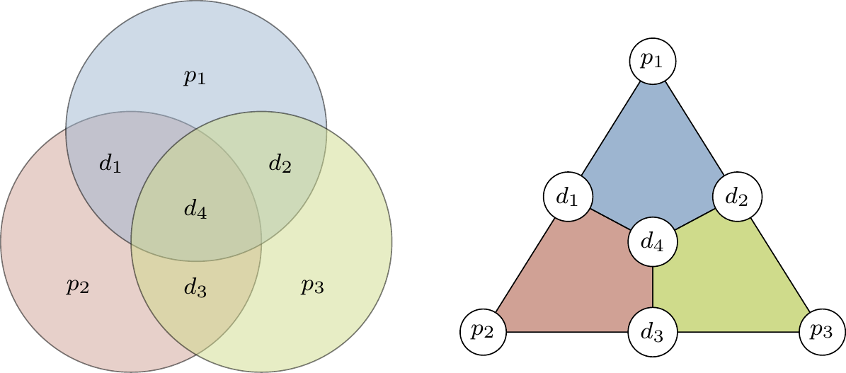
Image source: Qubit Guide - Introduction to Quantum Information Science
This Venn diagram shows how the three parity bits (p1, p2, p3) each cover different subsets of data bits (d1, d2, d3, d4). Each colored circle represents one parity bit’s coverage.
When the receiver decodes the message, it recalculates each parity bit. If all parity checks pass, the data is error-free. If some checks fail, the pattern reveals exactly which bit is wrong. The position of the error is encoded in the syndrome—a binary number formed by the failing parity checks.
For example, if parity bits 1 and 4 fail but bit 2 passes, the syndrome is 101 binary = 5 decimal. The error is at position 5. Flip that bit, and you’ve corrected the error.
The Hamming(7,4) code has a minimum distance of 3, allowing single-bit correction. But it can also detect (though not correct) two-bit errors. This makes it a SECDED code—Single Error Correction, Double Error Detection—which is exactly what most ECC memory uses today.
Shannon’s Limit: The Theoretical Boundary
In 1948, Claude Shannon published “A Mathematical Theory of Communication,” establishing the theoretical limits of error correction. His noisy-channel coding theorem states that for any communication channel with capacity $C$, it’s possible to transmit information at rate $R < C$ with arbitrarily low error probability.
Channel capacity depends on bandwidth and signal-to-noise ratio:
$$C = B \log_2\left(1 + \frac{S}{N}\right)$$Shannon’s theorem doesn’t tell us how to construct optimal codes—it only proves they exist. For decades, engineers created codes that fell far short of this theoretical limit. The gap between practical codes and Shannon’s limit was measured in decibels of signal-to-noise ratio.
It wasn’t until the 1990s, with the invention of turbo codes and the rediscovery of LDPC codes, that practical implementations began approaching Shannon’s limit. Today’s 5G and WiFi 6 systems operate within a fraction of a decibel of the theoretical optimum.
Reed-Solomon: Algebra to the Rescue
While Hamming codes work at the bit level, Reed-Solomon codes operate on symbols—typically bytes. Developed by Irving Reed and Gustave Solomon in 1960, these codes exploit the mathematics of polynomials over finite fields (Galois fields).
The key insight: a polynomial of degree $k-1$ is uniquely determined by any $k$ points on it. If you evaluate such a polynomial at $n$ points where $n > k$, you have redundancy—the extra points are consistent only if no errors occurred.
For a Reed-Solomon RS(n,k) code:
- You encode $k$ data symbols into $n$ transmitted symbols
- The code can correct up to $(n-k)/2$ symbol errors
- Symbol errors can be wrong values or complete erasures

Image source: Tom Verbeure - Reed-Solomon Error Correcting Codes from the Bottom Up
This graph shows how a polynomial is uniquely defined by any $n$ points. If some points are corrupted, the polynomial can still be reconstructed from the remaining correct points.
Reed-Solomon codes have a remarkable property: they can correct burst errors efficiently. Where Hamming codes correct random single-bit errors, Reed-Solomon excels at correcting concentrated damage—a scratch on a CD, a patch of static in satellite transmission. This makes them ideal for storage media and wireless communication.
The mathematics involve finite field arithmetic. In GF(256), the field of 256 elements used in most Reed-Solomon implementations, addition is XOR, and multiplication follows special rules defined by a primitive polynomial. This allows efficient hardware implementation while maintaining algebraic properties.
block-beta
    columns 7
    block:input:7
        A["k data symbols"]
    end
    space:7
    block:encode:7
        B["Message Polynomial<br/>m(x)"]
        C["Multiply by<br/>x^(n-k)"]
        D["Divide by<br/>Generator g(x)"]
        E["Remainder r(x)"]
    end
    space:7
    block:output:7
        F["Codeword: m(x)·x^(n-k) - r(x)"]
        G["k data symbols"]
        H["n-k parity symbols"]
    end
The diagram above shows the systematic encoding process for Reed-Solomon codes. The original data symbols appear unchanged in the codeword, with parity symbols appended.
From CDs to QR Codes: Reed-Solomon in Action
The compact disc, introduced in 1982, was the first mass-market application of Reed-Solomon codes. The Cross-Interleaved Reed-Solomon Code (CIRC) used two Reed-Solomon codes in sequence with interleaving between them. The result: a CD can withstand a 2.5mm scratch and still play perfectly. That’s approximately 4,000 consecutive bits of damage, corrected on the fly by the player’s decoder.
QR codes use four levels of Reed-Solomon error correction, specified by the ISO/IEC 18004 standard:
| Level | Data Capacity Reduction | Correctable Damage |
|---|---|---|
| L (Low) | ~7% | ~7% of codewords |
| M (Medium) | ~15% | ~15% of codewords |
| Q (Quartile) | ~25% | ~25% of codewords |
| H (High) | ~30% | ~30% of codewords |
At Level H, a QR code can have nearly 30% of its area damaged or obscured and still decode correctly. The Reed-Solomon decoder reconstructs the original message from the surviving 70%.
The relationship between redundancy and correction capability is linear for Reed-Solomon: to correct $t$ symbol errors, you need $2t$ redundant symbols. This is optimal among codes that correct symbol errors—the Singleton bound proves you can’t do better.
ECC Memory: When Your RAM Lies to You
Every second, cosmic rays strike Earth’s atmosphere, creating showers of secondary particles. Some of these particles—high-energy neutrons—pass through silicon chips, occasionally flipping a bit in your computer’s memory. Google’s study of DRAM errors across thousands of servers found error rates hundreds of times higher than manufacturers’ specifications, with approximately 8% of DIMMs experiencing errors per year.
ECC memory uses a Hamming variant called SECDED (Single Error Correction, Double Error Detection). For every 64 bits of data, 8 bits of ECC are stored—about 12.5% overhead. The code can:
- Correct any single-bit error
- Detect any double-bit error
- Detect (though not correct) most multi-bit errors
When ECC memory detects an uncorrectable error, it triggers a machine check exception. The system halts rather than proceeding with corrupted data. This is preferable to silent corruption, where incorrect results propagate through calculations undetected.
A 2009 study by Wisconsin researchers found that without ECC, memory errors would corrupt data silently in many systems. They estimated that a system with 10GB of RAM without ECC would experience a detectable memory error every 2.7 hours on average. With ECC, these errors are either corrected or cause controlled system halts.
The overhead of ECC has decreased over time. Early systems used 8 bits of ECC for 32 bits of data (25% overhead). Modern systems use 8 bits for 64 bits (12.5% overhead). Future systems with 128-bit data paths could use 9 bits (7% overhead), approaching the theoretical minimum.
Deep Space: Talking Across Billions of Kilometers
Voyager 1, launched in 1977, is now over 24 billion kilometers from Earth. Its 22.4-watt transmitter broadcasts at about 160 bits per second. The signal arrives at Earth with the power of a billionth of a billionth of a watt—weaker than a watch battery. How does any data survive the journey?
Error correction is the answer. Voyager uses concatenated codes: a convolutional code inner layer and a Reed-Solomon outer layer. The Reed-Solomon code—specifically RS(255, 223)—can correct up to 16 byte errors per 255-byte block. The convolutional code adds additional protection against random bit errors.
The improvement from error correction is dramatic. Without coding, the bit error rate at Voyager’s distance would be approximately 5%. With the concatenated code, it drops to about $10^{-6}$—one error per million bits. This 50,000x improvement in error rate comes at the cost of reduced data rate (the redundancy takes up bandwidth), but the trade-off is overwhelmingly favorable.
Voyager originally used a simpler Golay code for imaging data. In 1982, engineers uploaded new software to switch to Reed-Solomon, which provided 50 times better error correction with 5 times less overhead. This mid-mission upgrade demonstrates the power of Reed-Solomon coding—and the foresight of building reprogrammable spacecraft.
Modern Codes: Approaching Shannon’s Limit
For decades, practical codes fell short of Shannon’s theoretical limit by 2-3 dB. This gap mattered: at a given error rate, it meant transmitting 50-100% more power or accepting significantly higher error rates. Two breakthroughs in the 1990s changed everything.
Turbo Codes, developed at France Telecom in 1993, combine two convolutional codes with an interleaver and use iterative decoding. The decoder passes soft probability estimates between the two component decoders, refining the solution with each iteration. After 8-18 iterations, turbo codes approach within 0.5 dB of Shannon’s limit.
Low-Density Parity-Check (LDPC) Codes were invented by Robert Gallager in 1962 but were forgotten until their rediscovery in 1996. LDPC codes use a sparse parity-check matrix—a matrix with mostly zeros and few ones. This sparsity enables efficient iterative decoding similar to turbo codes.
Modern implementations of LDPC codes approach within 0.0045 dB of Shannon’s limit—virtually optimal. LDPC is now used in:
- 5G NR (New Radio) for data channels
- WiFi 6 (802.11ax)
- DVB-S2 satellite broadcasting
- SSD controllers for NAND flash
The shift from Reed-Solomon to LDPC in 5G reflects a fundamental trade-off. Reed-Solomon excels at burst errors but has higher overhead for the same correction capability. LDPC provides better performance on channels with random errors—which describes most wireless links—at the cost of more complex decoding.
gantt
    title Evolution of Error Correction Codes
    dateFormat YYYY
    section Early Codes
    Parity Bits              :1947, 5y
    Hamming Codes            :1950, 10y
    Reed-Solomon             :1960, 15y
    section Modern Codes
    LDPC Codes (Gallager)    :1962, 3y
    section Renaissance
    Turbo Codes              :1993, 3y
    LDPC Rediscovered        :1996, 10y
    section Deployment
    3G/4G (Turbo)            :2001, 15y
    5G (LDPC)                :2018, 8y
This timeline shows the development and deployment of major error correction codes, from Hamming’s original work to modern 5G systems.
The Trade-off Triangle
Every error correction code involves trade-offs between three parameters:
- Rate ($k/n$): The ratio of data bits to total bits. Higher rate means less overhead but weaker correction.
- Distance: The minimum Hamming distance between codewords. Greater distance means more errors can be corrected.
- Complexity: The computational cost of encoding and decoding. More powerful codes often require more computation.
Shannon’s theorem establishes the fundamental trade-off between rate and error probability for a given channel. For a channel with capacity $C$, you can’t transmit reliably at rate $R > C$. The art of code design is pushing as close to this boundary as possible while keeping complexity manageable.
Reed-Solomon codes are maximum distance separable (MDS)—they achieve the maximum possible distance for their rate. But they weren’t designed with iterative decoding in mind. Modern codes like LDPC sacrifice the MDS property for the ability to approach Shannon’s limit through iterative decoding.
For practical systems, decoding latency matters as much as error correction capability. A code that can correct more errors but requires 100ms to decode may be useless for real-time communication. This is why different applications use different codes:
| Application | Typical Code | Key Requirement |
|---|---|---|
| ECC Memory | Hamming SECDED | Low latency, hardware simplicity |
| Storage (SSD) | LDPC/BCH | High correction, some latency tolerance |
| Optical Media | Reed-Solomon | Burst error correction |
| Satellite | Concatenated RS + Convolutional | Maximum correction |
| 5G Data | LDPC | Near-Shannon performance |
| 5G Control | Polar | Low latency, small blocks |
When Error Correction Fails
No code can correct unlimited errors. When the error correction capability is exceeded, one of two things happens:
Detected failure: The decoder recognizes that correction is impossible. The system can request retransmission or flag the data as corrupted. This is the safe failure mode.
Undetected error: The decoder produces a wrong answer that passes all validity checks. This is catastrophic—the system proceeds with corrupted data, potentially propagating errors to subsequent calculations.
The probability of undetected error decreases exponentially with the code’s distance. For a Hamming code with distance 3, undetected errors require at least 3 bit flips in exactly the right pattern. For Reed-Solomon RS(255,223), undetected errors require at least 33 byte errors in a specific pattern—a astronomically unlikely event for most channels.
But for critical systems, even this low probability may be unacceptable. Safety-critical systems often use multiple independent error checks: CRC for detection, ECC for correction, checksums for validation. The probability of all checks failing simultaneously is the product of their individual failure probabilities—a vanishingly small number.
The Hidden Infrastructure
Error correction codes represent one of computing’s invisible triumphs. They work silently, constantly, everywhere. When you stream a video, LDPC codes protect against wireless interference. When you save a file, BCH or LDPC codes correct flash memory errors. When you scan a QR code, Reed-Solomon reconstructs the message from partial data.
Richard Hamming couldn’t have imagined the scope of his invention’s impact. His frustration with a weekend computer crash led to mathematical structures that now protect virtually every digital transmission. The next time your WiFi connection persists through interference, or your scratched DVD still plays, or your server runs for years without a memory error—thank the mathematicians who figured out how to make data resilient against a noisy universe.
References
-
Hamming, R. W. (1950). “Error Detecting and Error Correcting Codes.” Bell System Technical Journal, 29(2), 147-160.
-
Reed, I. S., & Solomon, G. (1960). “Polynomial Codes Over Certain Finite Fields.” Journal of the Society for Industrial and Applied Mathematics, 8(2), 300-304.
-
Shannon, C. E. (1948). “A Mathematical Theory of Communication.” Bell System Technical Journal, 27(3), 379-423.
-
Berrou, C., Glavieux, A., & Thitimajshima, P. (1993). “Near Shannon Limit Error-Correcting Coding and Decoding: Turbo-Codes.” IEEE International Conference on Communications.
-
Gallager, R. G. (1962). “Low-Density Parity-Check Codes.” IRE Transactions on Information Theory, 8(1), 21-28.
-
Schroeder, B., Pinheiro, E., & Weber, W.-D. (2009). “DRAM Errors in the Wild: A Large-Scale Field Study.” ACM SIGMETRICS Performance Evaluation Review.
-
Wikipedia. (2025). Hamming code. Retrieved from https://en.wikipedia.org/wiki/Hamming_code
-
Wikipedia. (2025). Reed–Solomon error correction. Retrieved from https://en.wikipedia.org/wiki/Reed%E2%80%93Solomon_error_correction
-
DENSO WAVE. (2025). Error correction feature. Retrieved from https://www.qrcode.com/en/about/error_correction.html
-
Verbeure, T. (2022). “Reed-Solomon Error Correcting Codes from the Bottom Up.” Retrieved from https://tomverbeure.github.io/2022/08/07/Reed-Solomon.html
-
Estévez, D. (2021). “Voyager 1 and Reed-Solomon.” Retrieved from https://destevez.net/2021/12/voyager-1-and-reed-solomon/
-
NASA JPL. (2020). “Voyager Telecommunications.” DESCANSO Series. Retrieved from https://descanso.jpl.nasa.gov/DPSummary/Descanso4--Voyager_ed.pdf
-
MIT News. (2010). “Explained: The Shannon limit.” Retrieved from https://news.mit.edu/2010/explained-shannon-0115
-
Qubit Guide. (2025). “The Hamming code.” Retrieved from https://qubit.guide/14.1-the-hamming-code
-
Cardinal Peak. (2025). “Low-Density Parity Check (LDPC) Codes for Modern Communications.” Retrieved from https://www.cardinalpeak.com/blog/low-density-parity-check-for-modern-communication-systems
-
Cook, J. D. (2025). “Advantages of Reed-Solomon codes over Golay codes.” Retrieved from https://www.johndcook.com/blog/2025/03/24/reed-solomon-golay/
-
Lin, S., & Costello, D. J. (2004). Error Control Coding (2nd ed.). Pearson.
-
MacWilliams, F. J., & Sloane, N. J. A. (1977). The Theory of Error-Correcting Codes. North-Holland.