In 1961, Les Earnest at MIT built the first spell checker as part of a cursive handwriting recognition system. His program used a list of just 10,000 common words, comparing each handwritten recognition result against the dictionary. The system was rudimentary, but it established a pattern that would repeat for decades: spell checking is fundamentally a string matching problem, and the challenge lies in making it fast enough to be useful.
By 1971, Ralph Gorin at Stanford had created a significantly more sophisticated system called SPELL. Instead of simple word lookup, Gorin’s program could suggest corrections by analyzing the structure of misspelled words. The program understood that “speling” might be “spelling” with a missing letter, and “acommodate” might be “accommodate” with a deleted character. This was the birth of intelligent spelling correction, built on algorithms that would eventually find their way into every word processor, search engine, and smartphone keyboard.
The problem these early systems solved is deceptively complex. When you type “definately” instead of “definitely,” a spell checker must somehow understand that these two strings are close enough to be related. But “close” is not a simple concept in computer science. The number of possible English words is around 170,000 in common usage, and for any misspelling, there might be dozens of plausible corrections. The challenge is finding the right ones—and doing it in milliseconds.
The Mathematical Foundation: Edit Distance
At the heart of every spell checker lies a concept called edit distance, formalized by Soviet mathematician Vladimir Levenshtein in 1965. The Levenshtein distance between two strings is the minimum number of single-character edits—insertions, deletions, or substitutions—required to transform one string into the other.
Consider “kitten” and “sitting.” The transformation requires three operations:
- Substitute “k” with “s” → “sitten”
- Substitute “e” with “i” → “sittin”
- Insert “g” at the end → “sitting”
The Levenshtein distance is 3. This number provides an objective measure of similarity between any two strings, regardless of language or context.
The mathematical definition uses a recursive formulation. For two strings $a$ and $b$, the Levenshtein distance $\text{lev}(a, b)$ is defined as:
$$\text{lev}(a, b) = \begin{cases} |a| & \text{if } |b| = 0 \\ |b| & \text{if } |a| = 0 \\ \text{lev}(\text{tail}(a), \text{tail}(b)) & \text{if } a[0] = b[0] \\ 1 + \min \begin{cases} \text{lev}(\text{tail}(a), b) \\ \text{lev}(a, \text{tail}(b)) \\ \text{lev}(\text{tail}(a), \text{tail}(b)) \end{cases} & \text{otherwise} \end{cases}$$where $\text{tail}(s)$ denotes the string $s$ with its first character removed.
The Wagner-Fischer Algorithm: Dynamic Programming in Action
The naive recursive implementation of Levenshtein distance has exponential time complexity because it recalculates the same subproblems repeatedly. In 1974, Robert Wagner and Michael Fischer published a dynamic programming solution that computes edit distance in $O(mn)$ time, where $m$ and $n$ are the lengths of the two strings.
The algorithm builds a matrix where each cell $d[i][j]$ represents the edit distance between the first $i$ characters of string $a$ and the first $j$ characters of string $b$. The matrix is filled row by row:
for i from 0 to m:
    d[i][0] = i  // deletion cost
for j from 0 to n:
    d[0][j] = j  // insertion cost

for i from 1 to m:
    for j from 1 to n:
        if a[i-1] == b[j-1]:
            substitutionCost = 0
        else:
            substitutionCost = 1
        d[i][j] = min(
            d[i-1][j] + 1,        // deletion
            d[i][j-1] + 1,        // insertion
            d[i-1][j-1] + substitutionCost  // substitution
        )
The final answer sits in $d[m][n]$, the bottom-right corner of the matrix.

Image source: Wikipedia - Levenshtein distance
This algorithm works well for comparing two strings, but spell checking requires comparing one misspelled word against an entire dictionary. With 170,000 words and an average word length of 8 characters, checking every dictionary entry against a 10-character misspelling would require roughly $170,000 \times 10 \times 8 = 13.6$ million operations—feasible but not fast enough for real-time correction.
Damerau-Levenshtein: The Transposition Problem
In 1964, Frederick Damerau observed that over 80% of human spelling errors are single-character errors: one insertion, deletion, substitution, or transposition of adjacent characters. The classic Levenshtein distance handles the first three but treats transpositions as two separate substitutions.
Consider “form” and “from.” Levenshtein distance would compute this as 2 (substitute “o” with “r”, then “r” with “o”). But intuitively, this is a single transposition of adjacent characters. The Damerau-Levenshtein distance captures this, returning 1.
The modification adds a fourth operation to the recurrence:
$$\text{DamerauLevenshtein}(a, b) = \min \begin{cases} \text{Levenshtein operations} \\ \text{lev}(a[0..i-2], b[0..j-2]) + 1 & \text{if } a[i] = b[j-1] \text{ and } a[i-1] = b[j] \end{cases}$$This captures the intuition that “teh” → “the” is a simpler transformation than “teh” → “tah” → “the.”
Peter Norvig’s Elegant Probabilistic Approach
In 2007, Peter Norvig, then Director of Research at Google, published a remarkably simple spell corrector that achieved 80-90% accuracy in just 21 lines of Python. The elegance lies not in the algorithm itself but in how it combines edit distance with probabilistic language modeling.
Norvig’s approach works in two phases. First, it generates all possible corrections within a certain edit distance of the misspelled word. For edit distance 1, this means:
- Deletions: remove one character (n possibilities)
- Transpositions: swap adjacent characters (n-1 possibilities)
- Replacements: replace one character with another (26n possibilities)
- Insertions: insert one character (26(n+1) possibilities)
For a 9-letter word, this generates about 114,000 candidate corrections.
Second, it selects the candidate with the highest probability given the context. Using Bayes’ theorem:
$$P(\text{correction}|\text{typo}) \propto P(\text{typo}|\text{correction}) \times P(\text{correction})$$The probability $P(\text{correction})$ comes from word frequency in a large corpus—common words like “the” are more likely corrections than rare words like “thesaurus.” The error model $P(\text{typo}|\text{correction})$ is simplified to assume all edit distance 1 corrections are equally likely, all edit distance 2 corrections are less likely, and so on.
def correction(word):
    return max(candidates(word), key=P)

def candidates(word):
    return (known([word]) or
            known(edits1(word)) or
            known(edits2(word)) or
            [word])

def known(words):
    return set(w for w in words if w in WORDS)
The brilliance of Norvig’s approach is its simplicity: generate plausible corrections, filter by known words, pick the most frequent. But for large dictionaries, generating 114,000 candidates and checking each against a dictionary is still computationally expensive.
BK-Trees: Exploiting Metric Space Properties
In 1973, Burkhard and Keller proposed a tree data structure specifically designed for approximate string matching. The BK-tree exploits a fundamental property of edit distance: it satisfies the triangle inequality.
$$d(a, c) \leq d(a, b) + d(b, c)$$This means that if we know the distance from a query word to some node in the tree, we can prune entire subtrees that cannot possibly contain closer matches.
A BK-tree is built by selecting an arbitrary word as the root. Each child edge is labeled with the edit distance from the parent. To insert a new word, compute its distance from the root, then follow the edge with that distance. If no such edge exists, create a new child.
Searching works by exploiting the triangle inequality. If we’re looking for words within distance 2 of a query, and we find that the root is distance 4 away, we can immediately skip all children connected by edges labeled outside the range $[2, 6]$. Any word at distance 7 or more from the root cannot possibly be within distance 2 of our query.

Image source: Wikipedia - BK-tree
The search complexity is $O(\log n)$ for evenly distributed data, though worst-case performance can degrade to $O(n)$ for pathological inputs. For spell checking applications, BK-trees reduce the number of edit distance calculations by orders of magnitude compared to brute-force approaches.
SymSpell: The 1000x Speedup
In 2012, Wolf Garbe introduced the Symmetric Delete algorithm, which achieved speeds 1000x faster than Norvig’s approach for edit distance 2 and over 1,000,000x faster for edit distance 3. The key insight is brilliantly counterintuitive: instead of generating all possible corrections at search time, precompute partial corrections at index time.
The algorithm exploits the symmetry of edit distance. If edit distance between two words is 1, then either:
- One word has one extra character (insertion), or
- The other word has one extra character (deletion), or
- Both words have the same length with one different character (substitution)
Instead of generating all insertions, deletions, substitutions, and transpositions from the misspelled word, SymSpell generates only deletions. This works because:
- If the correct word is an insertion of the misspelling, deleting that character from the correct word yields the misspelling
- If the correct word is a deletion of the misspelling, the misspelling itself already contains the correct word
- Substitutions and transpositions can be expressed as combinations of deletions and insertions
The precomputation step generates all deletion variants of every dictionary word. For maximum edit distance 2 and average word length 5, each word generates about 15 deletion variants. A 100,000-word dictionary produces roughly 1.5 million deletion entries.
At search time, generate deletion variants of the input word and look them up in a hash table. For a 9-letter word with edit distance 2, this produces just 36 candidates instead of 114,000.
Precomputation (one-time):
  For each dictionary word:
    Generate all delete variants (edit distance 1, 2, ...)
    Store in hash table with reference to original word

Search:
  Generate delete variants of input word
  Look up each variant in hash table
  Return matching dictionary words within max edit distance
The algorithm achieves $O(1)$ average-case lookup time, independent of dictionary size. This makes it practical for applications requiring sub-millisecond response times with concurrent users.
Tries: The Prefix Tree Advantage
While BK-trees and SymSpell focus on edit distance queries, another data structure excels at a different but related problem: prefix matching. The trie, invented independently by René de la Briandais in 1959 and Edward Fredkin in 1960, stores strings as paths through a tree where each node represents a character prefix.
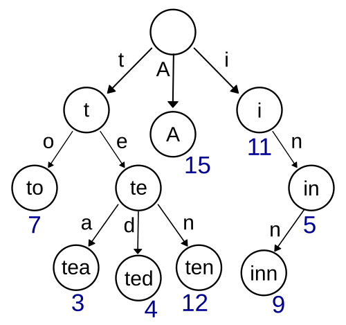
Image source: Wikipedia - Trie
Tries are ideal for autocomplete: as users type, the trie can instantly retrieve all words with a given prefix. But tries can also accelerate spell checking through a technique called depth-first search with early termination.
Starting from the root, traverse the trie while tracking the edit distance between the input word and the current path. If the edit distance exceeds the maximum allowed, backtrack and try a different branch. This avoids computing edit distances against dictionary words that cannot possibly match.
The search space is bounded by the trie structure rather than the dictionary size. For a 10-character input with maximum edit distance 2, the algorithm might explore thousands of trie nodes but avoid comparing against the remaining 99% of the dictionary.
Context-Aware Correction: Beyond Single Words
Traditional spell checkers operate on individual words in isolation. But many spelling errors create valid words that are incorrect in context—so-called “real-word errors.” Consider “I want to sale my car” versus “I want to sell my car.” Both “sale” and “sell” are valid words, but only one makes sense.
Context-aware spell checking uses language models to evaluate candidate corrections against their surrounding words. The probability of a word given its context can be estimated using n-gram models:
$$P(w_i | w_{i-n+1}, ..., w_{i-1}) \approx \frac{C(w_{i-n+1}, ..., w_i)}{C(w_{i-n+1}, ..., w_{i-1})}$$where $C(\cdot)$ denotes the count of an n-gram in a corpus.
Modern approaches use neural language models like BERT or GPT to compute context-dependent probabilities. These models capture semantic relationships that n-gram models miss, recognizing that “bank” means something different in “river bank” versus “bank account.”
The trade-off is computational cost. Neural language models require GPU acceleration for real-time performance, while simple n-gram models can run on any device. Most production spell checkers use a hybrid approach: fast edit-distance matching for candidate generation, followed by lightweight context scoring for disambiguation.
Phonetic Algorithms: Soundex and Beyond
Some spelling errors stem from phonetic confusion—users write what they hear. The Soundex algorithm, patented in 1918 and implemented in the 1930s for the U.S. Census, addresses this by encoding words based on their pronunciation.
Soundex reduces words to a letter followed by three digits:
- Retain the first letter
- Replace consonants with digits based on phonetic groups:
- b, f, p, v → 1
- c, g, j, k, q, s, x, z → 2
- d, t → 3
- l → 4
- m, n → 5
- r → 6
- Remove vowels and h, w
- Keep first three digits (pad with zeros if needed)
“Robert” and “Rupert” both encode to “R163.” “Smith” and “Smythe” both encode to “S530.”
Soundex was designed for English names and performs poorly for other languages. The Metaphone algorithm, published by Lawrence Philips in 1990, improves upon Soundex by considering English spelling rules more carefully. Double Metaphone (2000) further refines the algorithm and handles multiple pronunciations of the same word.
Phonetic algorithms work best as a preprocessing step: generate phonetic codes for dictionary words, then use them as an additional matching criterion alongside edit distance.
Neural Approaches: Seq2Seq and Transformers
Deep learning has transformed many NLP tasks, and spell correction is no exception. Sequence-to-sequence models treat spelling correction as a translation problem: translate from “misspelled language” to “correct language.”
A typical architecture uses an encoder-decoder framework. The encoder processes the misspelled word character by character, producing a hidden state that captures the word’s structure. The decoder generates the corrected word one character at a time, attending to relevant encoder states at each step.
# Conceptual seq2seq for spell correction
class SpellCorrector(nn.Module):
    def __init__(self, vocab_size, hidden_size):
        self.encoder = nn.LSTM(hidden_size, hidden_size)
        self.decoder = nn.LSTM(hidden_size, hidden_size)
        self.attention = nn.MultiheadAttention(hidden_size, num_heads=4)
        self.output = nn.Linear(hidden_size, vocab_size)
Transformer-based models like T5 and ByT5 have achieved state-of-the-art results on spelling correction benchmarks. These models learn contextual character-level representations, enabling them to handle errors that edit-distance approaches cannot—such as homophone confusion or complex morphological errors.
The limitation is practical deployment. Neural models require significant memory and computation. A BERT-based spell checker might need 400MB of memory and 50ms inference time on a modern CPU—unacceptable for real-time typing correction on mobile devices.
Applications Beyond Spell Checking
The algorithms developed for spell checking have found applications far beyond their original purpose:
DNA Sequence Alignment: The Levenshtein distance directly maps to biological mutations—insertions, deletions, and substitutions of nucleotides. Bioinformatics tools like BLAST use variants of edit distance to compare genetic sequences, identifying evolutionary relationships and detecting mutations.
Record Linkage: When merging databases, determining whether “John Smith” and “J. Smith” refer to the same person requires fuzzy string matching. The same edit-distance algorithms power deduplication in data warehouses.
Search Engines: Typo-tolerant search uses spell correction to find relevant documents even when queries contain errors. Elasticsearch and Solr implement phonetic analyzers and n-gram matching based on these principles.
Optical Character Recognition: OCR systems produce character-level errors similar to human typing. Spell correction post-processing can improve OCR accuracy by 5-10% on degraded documents.
The Performance Trade-offs
Choosing a spell checking algorithm involves balancing accuracy, speed, and memory:
| Algorithm | Time Complexity | Memory | Accuracy | Best Use Case |
|---|---|---|---|---|
| Brute Force | $O(n \cdot m \cdot k)$ | $O(k)$ | Perfect | Small dictionaries |
| BK-Tree | $O(\log n \cdot m)$ | $O(n)$ | Perfect | Static dictionaries |
| SymSpell | $O(1)$ lookup | $O(n \cdot e)$ | Perfect | Large-scale production |
| Norvig | $O(k^e \cdot m)$ | $O(k)$ | High | Prototyping |
| Neural | $O(m^2)$ | $O(100\text{MB})$ | Highest | Context-heavy errors |
Where $n$ is dictionary size, $m$ is word length, $k$ is alphabet size, and $e$ is max edit distance.
For most applications, SymSpell provides the best balance: sub-millisecond latency, perfect recall within the edit distance bound, and reasonable memory usage. Neural models are reserved for specialized applications where context-aware correction is critical.
References
-
Levenshtein, V. I. (1966). Binary codes capable of correcting deletions, insertions, and reversals. Soviet Physics Doklady, 10(8), 707-710.
-
Wagner, R. A., & Fischer, M. J. (1974). The string-to-string correction problem. Journal of the ACM, 21(1), 168-173.
-
Burkhard, W. A., & Keller, R. M. (1973). Some approaches to best-match file searching. Communications of the ACM, 16(4), 230-236.
-
Norvig, P. (2007). How to write a spelling corrector. norvig.com.
-
Garbe, W. (2012). 1000x faster spelling correction algorithm. SeekStorm Blog.
-
Damerau, F. J. (1964). A technique for computer detection and correction of spelling errors. Communications of the ACM, 7(3), 171-176.
-
Philips, L. (1990). Hanging on the metaphone. Computer Language, 7(12), 39-43.
-
Fredkin, E. (1960). Trie memory. Communications of the ACM, 3(9), 490-499.
-
Berger, B., Waterman, M. S., & Yu, Y. W. (2021). Levenshtein distance, sequence comparison and biological database search. IEEE Transactions on Information Theory, 67(6), 3287-3294.