In 1986, David Rumelhart, Geoffrey Hinton, and Ronald Williams published a paper in Nature that would transform artificial intelligence. The paper, “Learning representations by back-propagating errors,” demonstrated that a mathematical technique from the 1970s could train neural networks orders of magnitude faster than existing methods. The speedup wasn’t incremental—it was the difference between a model taking a week to train and taking 200,000 years.
But backpropagation wasn’t invented in 1986. Its modern form was first published in 1970 by Finnish master’s student Seppo Linnainmaa, who described it as “reverse mode automatic differentiation.” Even earlier, Henry J. Kelley derived the foundational concepts in 1960 for optimal flight path calculations. What the 1986 paper achieved wasn’t invention—it was recognition. The authors demonstrated that this obscure numerical technique was exactly what neural networks needed.
The Problem That Seemed Impossible
Training a neural network means finding the weights and biases that minimize a cost function. For a network with millions of parameters, this requires computing millions of partial derivatives—how the cost changes when each individual parameter wiggles slightly.
Consider a network with 10 million parameters. Naively computing these derivatives through finite differences would require 10 million forward passes through the network. If each forward pass takes 10 milliseconds, computing a single gradient requires over 27 hours. Train for 100,000 iterations, and you’re looking at 300 years.
Backpropagation computes all 10 million derivatives in roughly the time of two forward passes—about 20 milliseconds. That’s a speedup of roughly 10 million times. The algorithm achieves this through a clever application of the chain rule that reuses intermediate computations.
Computational Graphs: Seeing Mathematics as a Network
To understand backpropagation, you need to visualize mathematical expressions as graphs. Consider the expression $e = (a + b) \times (b + 1)$. We can decompose this into intermediate steps:
$$c = a + b$$$$d = b + 1$$
$$e = c \times d$$
Each operation becomes a node in a directed acyclic graph. Arrows connect inputs to outputs, showing how values flow through the computation.
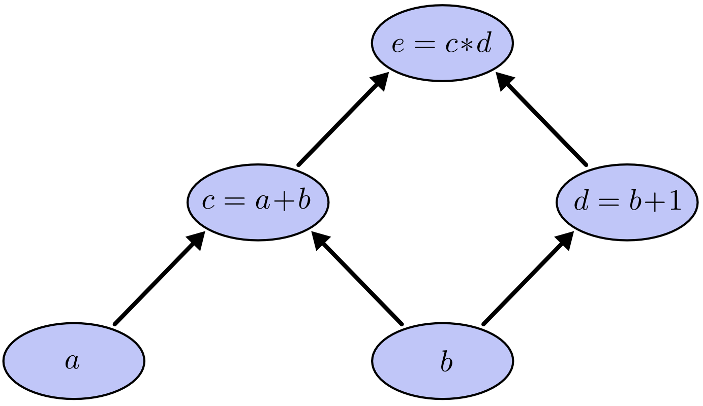
Image source: Colah’s Blog - Calculus on Computational Graphs
Now consider derivatives. If $a$ directly affects $c$, the partial derivative $\frac{\partial c}{\partial a} = 1$. If we want to know how $a$ affects $e$ (not directly connected), we multiply derivatives along all paths from $a$ to $e$:
$$\frac{\partial e}{\partial a} = \frac{\partial e}{\partial c} \times \frac{\partial c}{\partial a} = d \times 1 = d$$This is the chain rule, but visualized through graph traversal. The key insight: for nodes with multiple paths, we sum contributions from each path.
Forward-Mode vs Reverse-Mode Differentiation
When computing derivatives through a computational graph, two strategies emerge. Forward-mode differentiation starts at inputs and propagates forward, computing how one input affects all nodes. Reverse-mode differentiation starts at outputs and propagates backward, computing how all nodes affect one output.

Image source: Colah’s Blog - Calculus on Computational Graphs
For a function with many inputs and one output, reverse-mode differentiation is spectacularly efficient. One backward pass computes derivatives with respect to all inputs. For neural networks—which have millions of parameters (inputs) and one cost function (output)—this is exactly what we need.
The Four Fundamental Equations
Michael Nielsen’s classic treatment of backpropagation presents four equations that define the algorithm. These equations introduce an intermediate quantity $\delta^l_j$, the “error” in neuron $j$ of layer $l$, defined as:
$$\delta^l_j \equiv \frac{\partial C}{\partial z^l_j}$$where $z^l_j$ is the weighted input to the neuron and $C$ is the cost function.
Equation BP1 (Output Layer Error):
$$\delta^L_j = \frac{\partial C}{\partial a^L_j} \sigma'(z^L_j)$$This computes the error at the output layer. The first term measures how fast the cost changes with respect to output activations. The second term measures how fast the activation function changes at its input.
Equation BP2 (Error Propagation):
$$\delta^l = ((w^{l+1})^T \delta^{l+1}) \odot \sigma'(z^l)$$This propagates error backward. The transpose weight matrix moves error from layer $l+1$ to layer $l$. The Hadamard product (element-wise multiplication, denoted $\odot$) accounts for the activation function’s local derivative.
Equation BP3 (Bias Gradient):
$$\frac{\partial C}{\partial b^l_j} = \delta^l_j$$The gradient with respect to a bias equals the error at that neuron. This is computationally free once we’ve computed $\delta$.
Equation BP4 (Weight Gradient):
$$\frac{\partial C}{\partial w^l_{jk}} = a^{l-1}_k \delta^l_j$$The gradient with respect to a weight equals the input activation multiplied by the output error. This reveals a crucial insight: weights connected to low-activation neurons learn slowly.
The Algorithm in Practice
Backpropagation proceeds in three phases:
Forward Pass: Compute activations layer by layer from input to output, storing all intermediate values.
Backward Pass: Compute errors layer by layer from output to input using BP1 and BP2.
Gradient Computation: Use BP3 and BP4 to compute gradients from errors.
graph LR
    A[Input] --> B[Forward Pass]
    B --> C[Compute Loss]
    C --> D[Backward Pass]
    D --> E[Compute Gradients]
    E --> F[Update Weights]

    style A fill:#e1f5ff
    style C fill:#fff4e1
    style F fill:#e8f5e9
The computational cost? The backward pass requires roughly twice the computation of the forward pass. This comes from the matrix multiplications involved: computing $(w^{l+1})^T \delta^{l+1}$ requires the same operations as a forward pass through that layer, plus additional work for activation derivatives.
The Vanishing Gradient Problem
When backpropagation works, it works brilliantly. But as networks grew deeper in the 1990s and 2000s, researchers encountered a fundamental problem: gradients in early layers became exponentially small.
Consider a network with sigmoid activation functions. The sigmoid function $\sigma(x) = \frac{1}{1 + e^{-x}}$ has a maximum derivative of 0.25 at $x = 0$. When we multiply many small derivatives during backpropagation, the product shrinks exponentially. In a 10-layer network, if each layer contributes a factor of 0.25, the gradient reaching the first layer is multiplied by $0.25^{10} \approx 10^{-6}$.

Image source: Deep Learning Notes - Sigmoid Function
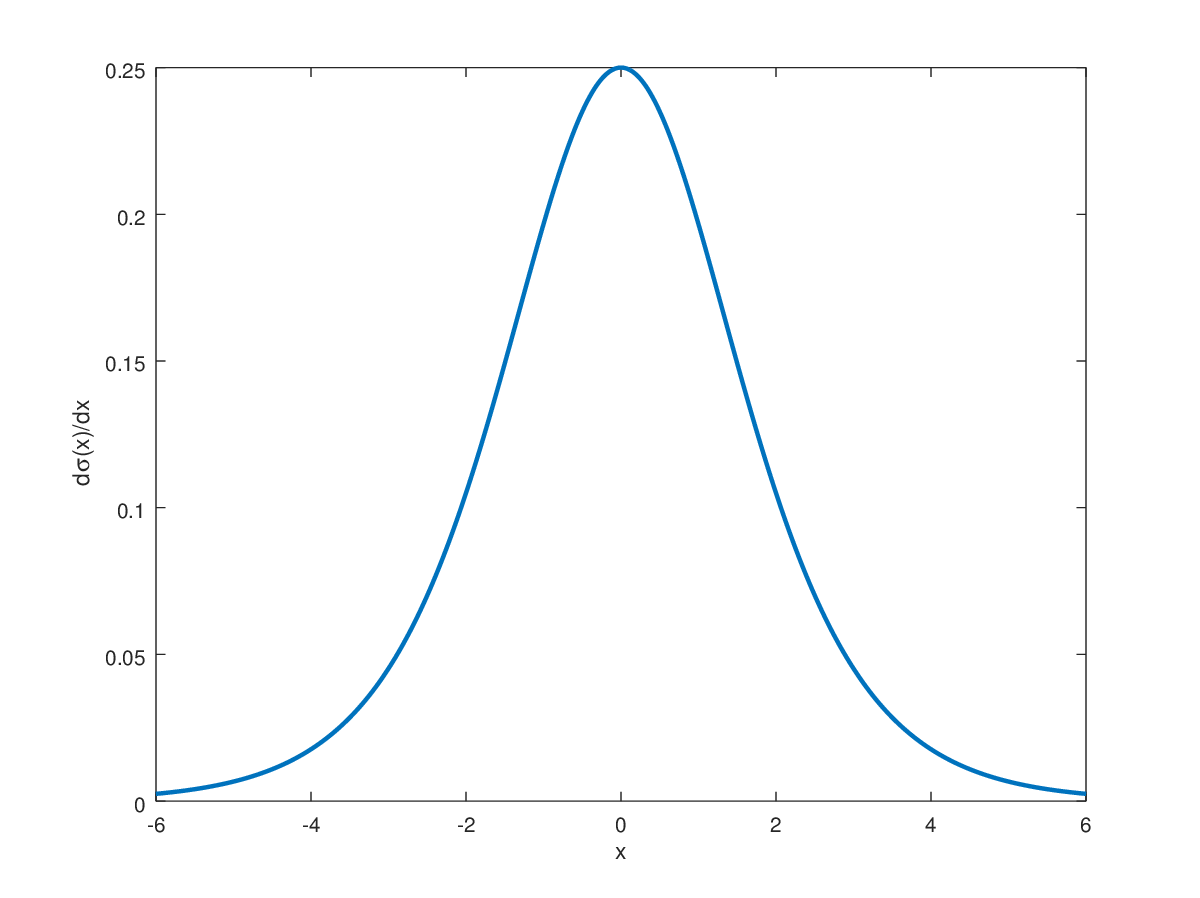
Image source: Deep Learning Notes - Sigmoid Derivative
Early layers receive nearly zero gradient and learn extremely slowly—or not at all. The network effectively stops learning features in its first layers.
Solutions That Changed Everything
The vanishing gradient problem stalled deep learning progress until several innovations converged around 2010-2012.
ReLU Activation: The Rectified Linear Unit, $f(x) = \max(0, x)$, has a derivative of 1 for positive inputs. No exponential decay. Gradients flow freely through active neurons. Simple, fast, and revolutionary.
Residual Connections: Introduced in 2015 for image recognition, skip connections add the input of a layer to its output: $y = f(x) + x$. During backpropagation, the gradient can flow directly through the identity shortcut, bypassing potentially vanishing paths. Networks with 152 layers became trainable.

Image source: Wikipedia - Residual Neural Network
Batch Normalization: Normalizing layer inputs stabilizes the distribution of activations, preventing them from reaching saturation regions where gradients vanish. This technique also allows higher learning rates.
Proper Initialization: Xavier initialization sets weights with variance $\frac{1}{n_{in}}$ where $n_{in}$ is the number of input connections. He initialization, designed for ReLU, uses $\frac{2}{n_{in}}$. These schemes ensure that activation variances remain stable across layers.
The Exploding Gradient Problem
The opposite problem also occurs. When gradients grow exponentially during backpropagation, weight updates become unstable. The network “explodes” numerically, with weights reaching extreme values.
Gradient clipping addresses this: when the gradient norm exceeds a threshold, scale it down. This simple technique prevents the most extreme updates while preserving gradient direction.
$$\nabla_{clipped} = \begin{cases} \nabla & \text{if } \|\nabla\| \leq \theta \\ \frac{\theta \nabla}{\|\nabla\|} & \text{otherwise} \end{cases}$$Modern Frameworks: Autograd
Modern deep learning frameworks—PyTorch, TensorFlow, JAX—implement backpropagation through automatic differentiation. The user defines a forward computation; the framework automatically constructs the computational graph and generates backward pass code.
PyTorch’s torch.autograd tracks operations on tensors with requires_grad=True. Each operation records how to compute its derivative. When .backward() is called, the framework traverses the graph in reverse order, applying chain rule operations.
The memory cost is substantial. Every intermediate activation must be stored for the backward pass. For large models, this dominates memory usage. A transformer model might store gigabytes of activations per training step.
Memory-Efficient Training
Training large models strains GPU memory. A 7-billion parameter model requires approximately 28 GB just to store parameters in FP32. Gradients require another 28 GB. Optimizer states—momentum and variance estimates for Adam—require 56 GB. Activations can require hundreds of gigabytes.
Gradient checkpointing addresses the activation memory problem. Instead of storing all intermediate activations, the framework stores only some (checkpoints). During backpropagation, it recomputes missing activations from the nearest checkpoint. This trades computation for memory: roughly 33% more compute for 50-70% less activation memory.
Mixed Precision Training
Modern GPUs offer substantial speedups and memory savings through FP16 (16-bit floating point) computation. But FP16 has limited range and precision—gradients often underflow to zero.
Loss scaling solves this. Before backpropagation, multiply the loss by a large constant (e.g., 65536). Gradients scale accordingly, avoiding underflow. After computing gradients, divide by the same scale. The framework automatically adjusts the scale factor during training.
Beyond Backpropagation
Backpropagation has limitations. It requires storing all intermediate activations. It computes gradients exactly, which isn’t always necessary. It assumes differentiable operations.
Alternative approaches are emerging. Forward-mode differentiation makes sense for functions with few inputs and many outputs. Implicit differentiation computes gradients without backpropagating through iterative algorithms. Randomized gradient estimators trade accuracy for memory.
Yet for most deep learning applications, backpropagation remains unbeaten. Its combination of exact gradients, efficient computation, and straightforward implementation has sustained it for nearly 40 years.
References
-
Rumelhart, D. E., Hinton, G. E., & Williams, R. J. (1986). Learning representations by back-propagating errors. Nature, 323(6088), 533-536.
-
Linnainmaa, S. (1970). The representation of the cumulative rounding error of an algorithm as a Taylor expansion of the local rounding errors. Master’s Thesis, University of Helsinki.
-
Kelley, H. J. (1960). Gradient theory of optimal flight paths. ARS Journal, 30(10), 947-954.
-
Nielsen, M. A. (2015). Neural Networks and Deep Learning. Determination Press.
-
Olah, C. (2015). Calculus on Computational Graphs: Backpropagation. Colah’s Blog.
-
He, K., Zhang, X., Ren, S., & Sun, J. (2016). Deep residual learning for image recognition. CVPR.
-
Glorot, X., & Bengio, Y. (2010). Understanding the difficulty of training deep feedforward neural networks. AISTATS.
-
Ioffe, S., & Szegedy, C. (2015). Batch normalization: Accelerating deep network training by reducing internal covariate shift. ICML.
-
Paszke, A., et al. (2019). PyTorch: An imperative style, high-performance deep learning library. NeurIPS.
-
Chen, T., et al. (2016). Training deep nets with sublinear memory cost. arXiv preprint arXiv:1604.06174.