When you create an index on a database table, have you ever wondered what data structure actually powers it? The answer is almost always a B+ tree. Not a hash table. Not a regular B-tree. Not a binary search tree. B+ trees have been the default index structure in nearly every major relational database for over five decades—MySQL, PostgreSQL, Oracle, SQL Server, and SQLite all use them. This isn’t coincidence or legacy inertia. It’s the result of fundamental trade-offs between disk I/O patterns, range query efficiency, and storage utilization.
The Problem with Binary Search Trees on Disk
To understand why B+ trees dominate, we need to first understand what goes wrong with simpler structures. A balanced binary search tree with 1 million elements has a height of approximately 20. That means finding any record requires traversing 20 nodes. In memory, this is fast—each node access is a few nanoseconds.
But databases don’t keep all data in memory. When data lives on disk, each node access becomes a disk read. A typical HDD can perform about 100-150 random I/O operations per second. At 10 milliseconds per random read, traversing a 20-level tree takes 200 milliseconds. That’s an eternity in computing terms.
Even on modern SSDs, which can handle 50,000+ IOPS, the problem persists. SSDs still perform better with sequential access than random access, and the random access penalty compounds across millions of lookups.
The fundamental insight is this: minimize the number of disk reads, not the number of comparisons. A B+ tree with a fanout of 100 can store 1 million records in just 3 levels. That’s 3 disk reads instead of 20—a 6x improvement that translates directly to query latency.
B-Tree vs B+ Tree: Where Did All the Data Go?
Both B-trees and B+ trees are self-balancing tree structures designed for disk storage. They share the core property of having multiple keys per node, which dramatically increases fanout and reduces tree height. But they differ in one crucial aspect: where the actual data lives.
In a B-tree, every node—internal and leaf—can store key-value pairs. When you traverse down the tree searching for a key, you might find your data at any level. This seems efficient: why go all the way to a leaf if you find what you need earlier?

Image source: Wikipedia - B+ tree
In a B+ tree, internal nodes store only keys—routing information that guides the search. All actual data resides in leaf nodes, which are linked together in a sorted doubly-linked list. This architectural choice has profound implications.
The space efficiency argument: Because internal nodes in B+ trees don’t store data, they can fit more keys per node. If each key is 8 bytes and each data pointer is 8 bytes, a B-tree node with 100 entries uses 1,600 bytes for keys and pointers. A B+ tree internal node with the same space can store 200 keys. More keys per node means higher fanout, which means shallower trees.
The range query argument: Consider a query like SELECT * FROM orders WHERE order_id BETWEEN 1000 AND 5000. In a B-tree, once you find the starting key, you must traverse the tree structure to find subsequent keys. The next key might be in a sibling node, a child node, or the same node—there’s no predictable pattern. This means random disk I/O for each key in the range.
In a B+ tree, all keys are in the sorted leaf list. You find the first key, then simply walk the linked list until you reach the upper bound. This transforms range queries from random access patterns into sequential access patterns. On HDDs, sequential reads are 10-100x faster than random reads. Even on SSDs, sequential access benefits from prefetching and reduced overhead.
Jeremy Cole’s analysis of InnoDB’s B+ tree implementation shows that a three-level B+ tree can index over 677 million records with each lookup requiring at most 3 disk reads. The same data in a B-tree with data in internal nodes would require more levels due to lower fanout.
Hash Indexes: Fast Lookups, Narrow Use Cases
If you only care about exact match queries—WHERE id = 42—hash indexes seem ideal. A well-implemented hash index provides O(1) average-case lookup, which beats the O(log n) of B+ trees. PostgreSQL offers hash indexes, and they can be 10-22% faster than B-tree indexes for pure equality lookups on large tables.
So why aren’t hash indexes the default?
No range queries: A hash function scrambles input values into seemingly random bucket positions. The values 100, 101, and 102 might hash to completely different buckets. There’s no way to find all values in a range without checking every bucket. For a database system that must support ORDER BY, BETWEEN, and comparison operators, this is a fatal limitation.
No prefix matching: Queries like WHERE name LIKE 'John%' can use a B+ tree index because it maintains sorted order. The database finds the first entry starting with “John” and scans forward. A hash index cannot help here—there’s no way to hash a prefix.
No ordering support: Hash indexes can’t help with ORDER BY clauses. The database must still sort the results after retrieval.
Collision handling overhead: Hash collisions are inevitable. When multiple keys hash to the same bucket, the database must search through them linearly. A poorly chosen hash function or unlucky data distribution can degrade performance dramatically.
Memory overhead for collision chains: Hash indexes often need overflow pages or linked lists to handle collisions, which increases storage requirements unpredictably.
The PostgreSQL documentation effectively recommends using B-tree indexes by default, resorting to hash indexes only when you fully understand their limitations and your workload consists purely of equality lookups.
The Fanout Calculation: Why Tree Height Matters
Let’s work through a concrete example. Consider a database with 100 million records, each indexed by a 4-byte integer primary key. Assume 8-byte pointers and a 16KB page size (the default in MySQL’s InnoDB).
B+ tree internal node: Can store approximately $\frac{16KB}{4 + 8} \approx 1,365$ key-pointer pairs. Let’s use 1,000 for a conservative estimate accounting for node headers.
Tree height calculation:
- Level 1 (root): 1,000 keys
- Level 2: 1,000 × 1,000 = 1,000,000 keys
- Level 3: 1,000 × 1,000 × 1,000 = 1,000,000,000 keys
A three-level B+ tree can index 1 billion records. Finding any record requires reading at most 3 pages: root, one internal node, and one leaf node. With a buffer pool caching the root and frequently-accessed internal nodes, most queries hit in 1-2 disk reads.
B-tree internal node: Must store keys plus data pointers. If each data record is 100 bytes, each entry in an internal node takes 104 bytes. A 16KB node can store only $\frac{16KB}{104} \approx 150$ entries.
Tree height calculation:
- Level 1: 150 keys
- Level 2: 150 × 150 = 22,500 keys
- Level 3: 150³ = 3,375,000 keys
- Level 4: 150⁴ = 506,250,000 keys
- Level 5: 150⁵ = 75 billion keys
For 100 million records, the B-tree needs 4-5 levels versus 3 for the B+ tree. Each additional level means one more disk read. At 10ms per read on HDD, that’s 10-20ms additional latency per query.
Sequential Access: The Hidden Performance Win
The linked leaf nodes in B+ trees enable a crucial optimization: sequential access patterns for range scans.
Consider a query fetching 1,000 consecutive records by primary key. In a B+ tree:
- Traverse to the first leaf (3 disk reads)
- Scan forward through leaf nodes (sequential reads)
In a B-tree without linked leaves:
- Traverse to find each record (up to 4 reads per record)
- Navigate tree structure for each subsequent key
The B+ tree approach transforms 4,000 random reads into approximately 3 random reads plus a sequential scan. On HDDs, sequential reads can achieve 100-200 MB/s while random reads top out at 1-2 MB/s. That’s a 100x throughput difference.
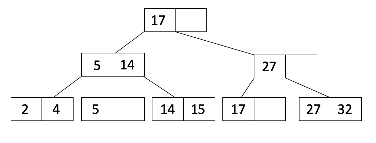
Image source: UC Berkeley CS186 - B+Trees
Even on SSDs, sequential access benefits from read-ahead prefetching and reduced command overhead. The storage controller can fetch adjacent pages speculatively, hiding latency effectively.
Disk Block Alignment: Why 4KB and 16KB Matter
B+ trees are designed around disk block boundaries. The typical approach is to make each B+ tree node exactly one disk block—or one database page, which is typically 4KB, 8KB, or 16KB depending on the database system.
This alignment is not arbitrary. It ensures that reading one node reads exactly one disk block—no more, no less. The operating system’s page cache, the storage device’s internal cache, and the database’s buffer pool all operate on block boundaries. When these align, every layer works efficiently.
A node smaller than a block wastes space. A node larger than a block requires multiple reads, potentially fragmenting across non-contiguous disk locations. The sweet spot is exactly matching the I/O granularity of the storage stack.
MySQL’s InnoDB uses a 16KB default page size, which it found provides good balance for most workloads. PostgreSQL uses 8KB. Oracle defaults to 8KB. The choice involves trade-offs:
Larger pages (16KB-64KB):
- More keys per node → shallower trees → fewer disk reads per lookup
- Better sequential scan performance for range queries
- Higher memory pressure in buffer pool
- More wasted space for partially-filled pages
Smaller pages (4KB-8KB):
- Better memory utilization
- Less wasted space in partially-filled pages
- Better for OLTP workloads with many small random accesses
- Deeper trees → potentially more disk reads
Research from Microsoft on page size selection shows that 8KB-16KB represents a sweet spot for traditional database workloads, balancing random access latency against sequential scan efficiency.
Covering Indexes: When You Don’t Need the Table
B+ trees enable a powerful optimization: the covering index. If all columns needed by a query exist in the index, the database can satisfy the query entirely from the index without accessing the table data.
Consider an index on (last_name, first_name) and a query:
SELECT first_name FROM users WHERE last_name = 'Smith'
The B+ tree leaf nodes contain both last_name and first_name. The database finds all entries with last_name = 'Smith' and returns first_name values directly. No table access needed.
This “index-only scan” can be 10-100x faster than fetching from the table, especially for queries matching many rows. The leaf nodes are contiguous, enabling sequential access, while the table data might be scattered across the disk.
PostgreSQL’s visibility map and index-only scans demonstrate this optimization in production. The database tracks which pages have only visible-to-all transactions, allowing it to skip table access entirely for recent data.
When Hash Indexes Actually Make Sense
Hash indexes aren’t useless—they’re specialized tools for specific workloads:
Session stores: Key-value lookups where you only ever query by exact session ID. No range queries, no ordering, just WHERE session_id = ?.
Lookup tables: Reference data where access is always by exact primary key, such as country codes, currency mappings, or configuration flags.
High-cardinality equality scans: When a column has millions of distinct values and queries are always equality comparisons, hash indexes can provide measurable performance gains.
PostgreSQL’s hash indexes received significant improvements in version 10, making them crash-safe and more performant. But the documentation still recommends B-tree for most use cases because hash indexes remain fundamentally limited to equality operations.
The rule of thumb: use B+ tree by default. Consider hash indexes only when your access patterns are provably limited to equality lookups and you’ve measured the performance benefit.
Write Amplification: The Hidden Cost
B+ trees aren’t without trade-offs. One significant issue is write amplification during node splits.
When a node overflows, it must split into two nodes and push a key up to the parent. This can cascade up the tree. A single insertion might cause multiple page writes: the two new leaf pages and each ancestor page up to the root.
For a B+ tree of height 3, a single insert could require 4 page writes (2 leaf splits + 2 internal node updates). This is where LSM trees (Log-Structured Merge trees) have an advantage—they’re optimized for write-heavy workloads by batching writes and performing sequential I/O.
However, B+ trees have compensating advantages for most transactional workloads:
- Predictable read performance: Any record is retrievable in bounded time
- No read amplification: Finding a record doesn’t require checking multiple sorted runs
- Simpler transaction semantics: Row-level locking is straightforward with B+ trees
The choice between B+ trees and LSM trees depends on your read/write ratio. For read-heavy or mixed workloads, B+ trees usually win. For write-heavy workloads with occasional reads, LSM trees may be better.
The Buffer Pool: Where B+ Trees Shine in Memory
Databases don’t read from disk for every query. They maintain a buffer pool—an in-memory cache of frequently-accessed pages. The buffer pool is where B+ tree performance truly excels.
Because B+ tree internal nodes are small and cache efficiently, a moderate buffer pool can cache the top several levels of the tree. For a 100 million record table, the root and all level-2 internal nodes might fit in a few megabytes. Once cached, queries only need to read leaf nodes from disk.
This caching behavior explains why database performance often improves dramatically after “warm-up”—the first few queries populate the buffer pool with frequently-used internal nodes, and subsequent queries become much faster.
The buffer pool also enables optimizations like:
- Dirty page batching: Multiple updates to the same page are coalesced before writing to disk
- Group commit: Multiple transactions’ changes to adjacent pages can be written together
- Adaptive hash indexing: The database can build in-memory hash indexes on top of frequently-accessed B+ tree paths
Summary
B+ trees dominate database indexing because they were designed for the specific constraints of disk-based storage: minimizing disk reads, enabling efficient range queries, and aligning with block-based I/O. The separation of routing information (internal nodes) from data (leaf nodes) maximizes fanout, reducing tree height. The linked leaf structure transforms range queries from random access patterns into sequential access patterns.
Hash indexes have their place for pure equality lookups, but their inability to support range queries, ordering, and prefix matching makes them unsuitable as a default. B-trees work but sacrifice the sequential access optimization that makes B+ trees superior for range scans.
The next time you create an index without specifying a type, know that you’re getting a B+ tree—a data structure that has survived five decades of computing evolution because it solves the fundamental problem better than any alternative: how to find data quickly when that data lives on disk.
References
- Bayer, R., McCreight, E. (1970). “Organization and maintenance of large ordered indices”. Proceedings of the ACM SIGFIDET Workshop.
- Comer, D. (1979). “The Ubiquitous B-Tree”. ACM Computing Surveys, 11(2), 121-137.
- Cole, J. (2013). “B+Tree index structures in InnoDB”. blog.jcole.us
- PostgreSQL Documentation. “Index-Only Scans and Covering Indexes”.
- UC Berkeley CS186. “B+Trees”. cs186berkeley.net
- CMU 15-445. “Tree Indexes”. Database Systems Course Notes.
- Microsoft Research. “Why 16K May Not Be the Right Answer for B-tree Page Size”.
- EnterprisedDB. “Are Hash Indexes Faster than Btree Indexes in Postgres?”
- PingCAP. “Understanding B-Tree and Hash Indexing in Databases”.