In 2013, Tomas Mikolov and his team at Google published a paper that would fundamentally change how machines understand language. They showed that by training a simple neural network to predict surrounding words, you could learn vector representations where “king” minus “man” plus “woman” approximately equals “queen.” This was the birth of modern word embeddings—a technique that compresses the meaning of words into dense numerical vectors.
A decade later, embeddings have become the backbone of virtually every AI application involving text. They power semantic search, recommendation systems, and the retrieval component of RAG (Retrieval-Augmented Generation) architectures. But as organizations deploy these systems at scale, many discover an uncomfortable truth: semantic search often fails in ways that are hard to predict and even harder to debug.
What Embeddings Actually Capture
At their core, embeddings are dimensionality reduction machines. They take discrete symbols—words, sentences, documents—and map them into a continuous vector space where similar meanings cluster together. The intuition is seductively simple: if two pieces of text have similar meanings, their vectors should be close together in this space.
Word2Vec accomplished this through two architectures: Continuous Bag of Words (CBOW) and Skip-gram. CBOW predicts a target word from its context, while Skip-gram does the reverse, predicting context words from a target. Despite their simplicity, these models learned remarkably sophisticated relationships. The vectors captured not just semantic similarity but analogical reasoning—the famous example being $\vec{king} - \vec{man} + \vec{woman} \approx \vec{queen}$.
Modern embedding models have evolved far beyond these early approaches. Transformer-based models like BERT generate contextual embeddings where the representation of a word changes based on the surrounding text. The word “bank” in “river bank” gets a different vector than “bank” in “investment bank.” Sentence transformers fine-tune these models using contrastive learning, training them to pull similar sentences closer together while pushing dissimilar ones apart.
The result is impressive: embed a query like “how do I reset my password” and a document containing “password reset instructions,” and the vectors will be nearly parallel. The angle between them—the cosine similarity—will approach 1.0, indicating high semantic similarity. This works reliably enough that cosine similarity has become the default metric for semantic search.

Image source: Pinecone
When Cosine Similarity Betrays You
Here’s the problem: cosine similarity measures the angle between vectors, but ignores their magnitude entirely. A vector with magnitude 0.001 pointing in direction $\theta$ has the same cosine similarity to another vector as a vector with magnitude 1000 pointing in the same direction. This invariance is often presented as a feature—it makes embeddings robust to scale variations. But it also discards potentially meaningful information.
Research has shown that embedding magnitude carries semantic signals. Longer vectors often correspond to more frequent words or more “confident” representations. When you normalize these vectors for cosine similarity, you’re throwing away information about how certain or informative a representation is.
A more subtle problem is anisotropy—the tendency of embeddings to cluster along dominant directions in the vector space. In an ideal embedding space, vectors would be uniformly distributed, pointing in all directions with equal probability. This property is called isotropy. In practice, transformer embeddings are highly anisotropic. They tend to occupy a narrow cone in the high-dimensional space, with most vectors pointing in similar directions.
Why does this matter? When all vectors cluster in a narrow cone, cosine similarity becomes a poor discriminator. Imagine everyone in a room standing in the same corner—even small differences in position become magnified in importance, while the overall structure loses meaning. Studies have shown that this anisotropy can cause BERT embeddings to perform poorly on semantic similarity tasks, despite the model’s strong performance on other NLP benchmarks.
The mathematics is unforgiving. In a 768-dimensional space (typical for BERT-base), if vectors occupy only a narrow cone, the effective dimensionality of the semantic space might be much lower. You’re not actually getting 768 degrees of freedom to represent meaning—you might only have 50 or 100 meaningful dimensions, with the rest contributing noise.
The Hubness Problem and Dimensional Curse
High-dimensional spaces behave counterintuitively. One phenomenon that surprises many practitioners is the “hubness problem.” In high-dimensional vector spaces, some points become hubs—they appear in the nearest-neighbor lists of many other points, while other points rarely appear in anyone’s nearest neighbors.
This isn’t a bug in your vector database. It’s a mathematical consequence of the concentration of measure in high dimensions. As dimensionality increases, distances between points become more uniform—the ratio of the distance to the nearest neighbor versus the distance to the farthest neighbor approaches 1. This makes nearest-neighbor search increasingly noisy.
The hubness problem has real consequences for recommendation and retrieval systems. Popular items become over-recommended, not because they’re genuinely more relevant, but because their embedding vectors happen to lie in a position that makes them “neighbors” to many query vectors. Meanwhile, genuinely relevant but less-connected items get buried.
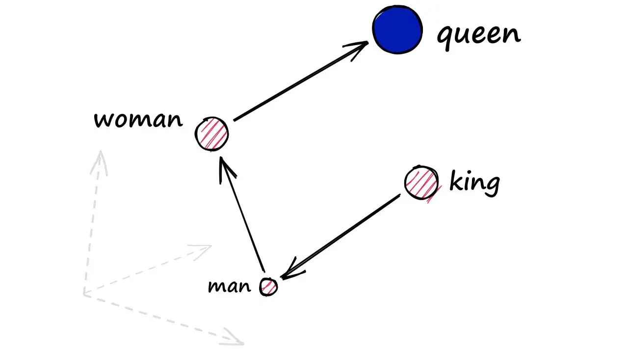
Image source: Pinecone
The Negation Problem
Perhaps the most frustrating failure mode of semantic search is its inability to handle negation. Query for “authentication WITHOUT OAuth” and semantic search will happily return documents about “authentication WITH OAuth.” The vectors are similar because the texts are similar—the negation doesn’t create enough distance in the embedding space.
This happens because embeddings are trained to capture co-occurrence patterns and semantic similarity. The words “with” and “without” often appear in similar contexts, discussing the same topics. Their embeddings end up close together. When you embed a query containing “without OAuth,” the resulting vector isn’t that different from one containing “with OAuth.”
The problem extends beyond simple negation. Queries that require exclusions, conditionals, or precise entity matching often fail. “Show me documents about Python, the programming language, not the snake” will return results about pythons (the snake) because the word “Python” dominates the embedding, and the disambiguation clause gets lost in the compression.
How Vector Search Actually Works
Understanding why semantic search fails requires understanding how vector databases find similar items. They don’t compare your query to every document—that would be far too slow for million-scale collections. Instead, they use approximate nearest neighbor (ANN) algorithms.
The most popular is Hierarchical Navigable Small World (HNSW). It builds a multi-layer graph where each node connects to its nearest neighbors. The top layers have sparse connections for fast traversal; the bottom layer has dense connections for accuracy. To search, you start at the top, greedily move toward the query, and descend layer by layer until you find the best matches.
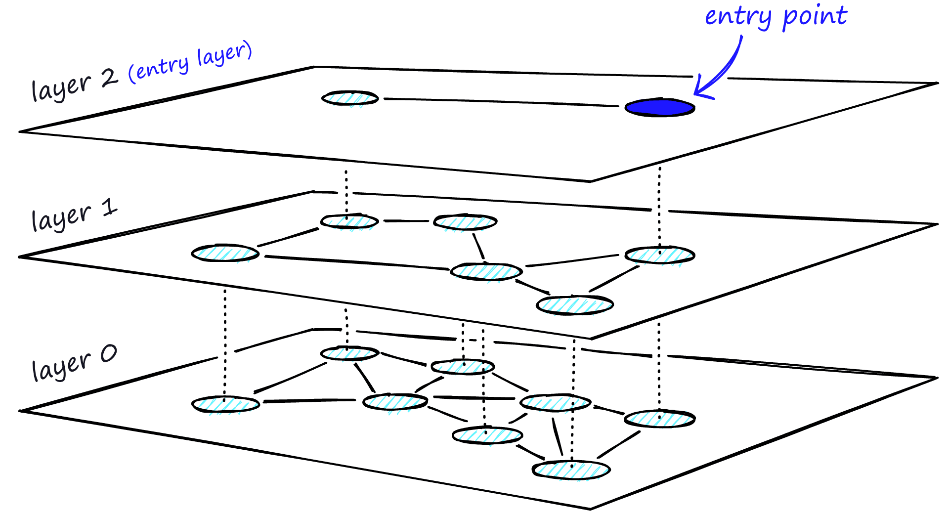
Image source: Pinecone
HNSW is fast—logarithmic time complexity—but it’s approximate. You might get the 10 most similar documents, or you might miss the true nearest neighbor because the graph traversal got stuck in a local minimum. The trade-off is controlled by parameters like M (connections per node) and ef (search depth). Higher values mean better recall but slower queries and more memory usage.
Another approach is Inverted File Index (IVF), which partitions the vector space into cells using clustering. Each document belongs to one cell centered around a centroid. During search, you only compare against documents in the nearest cells, dramatically reducing comparisons. The trade-off is the “edge problem”—if your query lands near a cell boundary, the true nearest neighbor might be in an adjacent cell you’re not searching.
Why Chunking Matters More Than You Think
Embedding quality depends critically on what you embed. In RAG systems, documents are typically split into chunks before embedding. The chunking strategy you choose can make or break retrieval performance.
Naive fixed-size chunking (e.g., 512 tokens) ignores semantic boundaries. A chunk might end mid-sentence or split a definition from its explanation. When you embed such chunks, you’re compressing incomplete or incoherent text, leading to noisy vectors.
Semantic chunking attempts to split at natural boundaries—paragraphs, sections, or topic transitions. But this introduces its own problems. Some chunks become too short to carry meaningful context; others become too long, diluting the specific information a query might seek. The embedding model was trained on specific text lengths; feeding it chunks that deviate from those lengths can degrade performance.
The chunking problem compounds with the “lost in the middle” phenomenon. Research shows that when documents are presented to an LLM, information in the middle of the context window is recalled less accurately than information at the beginning or end. If your retrieval returns 20 chunks and the most relevant one ends up in position 15, the LLM might ignore it entirely.
Hybrid Search: The Pragmatic Solution
Given these limitations, production systems rarely rely on pure vector search. The dominant approach is hybrid search—combining dense (embedding-based) retrieval with sparse (keyword-based) retrieval like BM25.
BM25 is a statistical ranking function that predates neural embeddings by decades. It ranks documents based on term frequency, inverse document frequency, and document length normalization. It has no understanding of semantics—if you search for “canine,” it won’t find documents about “dogs” unless they explicitly mention “canine.”
But BM25 excels where embeddings fail: exact term matching, handling rare words, and respecting query structure. A query for “OAuth WITHOUT SAML” will correctly exclude documents mentioning SAML because BM25 sees the explicit term negation.
Hybrid search combines both approaches, typically using Reciprocal Rank Fusion (RRF). You run parallel retrievals—semantic search via embeddings, keyword search via BM25—and merge the ranked lists. Documents that appear high in both lists get boosted; those that only appear in one list get downweighted.
The improvement can be dramatic. Studies show hybrid search consistently outperforms either approach alone, often by 10-20% in retrieval accuracy. The downside is complexity—you need to maintain both indexes and tune the fusion parameters.
Reranking: The Second Pass
Even hybrid search returns imperfect results. That’s where reranking comes in—a two-stage retrieval approach that’s become standard in production RAG systems.
In the first stage, you cast a wide net. Retrieve 50-100 candidate documents using fast, approximate methods like vector search or hybrid retrieval. These might include false positives—documents that are semantically similar to the query but not actually relevant.
In the second stage, you run a cross-encoder reranker on these candidates. A cross-encoder is a transformer model that takes both the query and a candidate document as input and produces a relevance score. Unlike bi-encoders (embedding models), cross-encoders can attend to interactions between query and document tokens—they can see that the document mentions “OAuth” and the query asks about “OAuth without SAML” and reason about whether it’s a match.

Image source: Pinecone
The trade-off is speed. Cross-encoders are 100-1000x slower than vector search. You can’t run them over your entire corpus. But you only need to run them on the small candidate set from the first stage, making the total latency acceptable.
The Geometry We Ignore
The deeper lesson is that embeddings are not magic. They’re lossy compressions that preserve some aspects of meaning while discarding others. The geometry of the embedding space—the concentration of vectors, their anisotropy, the hubness phenomenon—has real consequences for search quality.
As you build semantic search systems, remember that cosine similarity is a heuristic, not a truth measure. Two vectors being close doesn’t guarantee their texts are relevant; two vectors being far doesn’t guarantee their texts are unrelated. The embedding captures what it was trained to capture, which might not align with what your users are searching for.
The most robust systems acknowledge these limitations. They use hybrid retrieval to catch what embeddings miss. They rerank with cross-encoders to correct first-stage errors. They tune chunking strategies to match their document types and query patterns. And they measure—not just retrieval metrics like recall@k, but downstream metrics like answer quality and user satisfaction.
Semantic search works. But understanding why it fails is what separates toy demos from production systems.
References
- Mikolov, T., et al. (2013). Efficient Estimation of Word Representations in Vector Space. arXiv:1301.3781
- Devlin, J., et al. (2019). BERT: Pre-training of Deep Bidirectional Transformers for Language Understanding. NAACL-HLT 2019.
- Reimers, N., Gurevych, I. (2019). Sentence-BERT: Sentence Embeddings using Siamese BERT-Networks. EMNLP-IJCNLP 2019.
- Malkov, Y., Yashunin, D. (2016). Efficient and robust approximate nearest neighbor search using Hierarchical Navigable Small World graphs. IEEE TPAMI.
- Radovanovic, M., et al. (2010). Hubs in Space: Popular Nearest Neighbors in High-Dimensional Data. JMLR.
- Ethayarajh, K. (2019). How Contextual are Contextualized Word Representations? EMNLP-IJCNLP 2019.
- Muennighoff, N., et al. (2022). MTEB: Massive Text Embedding Benchmark. arXiv:2210.07316
- Liu, N., et al. (2023). Lost in the Middle: How Language Models Use Long Contexts. arXiv:2307.03172
- Neelakantan, A., et al. (2022). Text and Code Embeddings by Contrastive Pre-Training. arXiv:2201.10005
- Ethayarajh, K., et al. (2022). Is Anisotropy Really the Cause of BERT Embeddings Not Being Semantic? Findings of EMNLP 2022.