At 2:17 AM on a Tuesday, a major e-commerce platform’s API went down. The incident report later revealed the root cause: a misconfigured rate limiter had allowed a burst of requests through at exactly the boundary between two time windows, overwhelming downstream services. The platform had implemented a fixed window counter—the simplest rate limiting algorithm—and paid the price for its simplicity.
Rate limiting seems straightforward: allow N requests per time period. But the algorithm you choose determines not just whether your system survives traffic spikes, but how fairly it treats users, how much memory it consumes, and whether it creates new failure modes you never anticipated. The difference between algorithms isn’t academic—it’s the difference between a system that degrades gracefully and one that cascades into total failure.
The Fixed Window Counter: Simplicity With a Fatal Flaw
The fixed window counter divides time into discrete intervals—say, one-minute buckets—and counts requests within each. When a request arrives, increment the counter for the current window. If the count exceeds the limit, reject the request. At the end of the window, reset the counter to zero.
This approach has compelling advantages. Memory usage is minimal: one integer per user or API key. Implementation is trivial in any language. Redis makes it even easier with atomic increments and key expiration.
def allow_request(user_id, limit=100):
    window = current_minute()
    key = f"rate:{user_id}:{window}"
    count = redis.incr(key)
    if count == 1:
        redis.expire(key, 60)  # expire after 60 seconds
    return count <= limit
But consider what happens at window boundaries. A user limited to 100 requests per minute could send 100 requests at 11:59:59 and another 100 at 12:00:01—200 requests in two seconds. The rate limiter sees two separate windows and allows both bursts. This isn’t a theoretical concern; Cloudflare documented this exact pattern in their analysis of traffic patterns.

Image source: Cloudflare Blog
The boundary problem becomes severe at scale. An attacker coordinating requests across multiple accounts could synchronize their bursts to window boundaries, briefly overwhelming downstream services before the rate limiter catches up.
The Sliding Window Log: Precision at a Cost
The sliding window log solves the boundary problem by storing timestamps of every request. When a new request arrives, remove timestamps older than the time window, count the remaining entries, and decide whether to allow the request.
This approach is perfectly accurate. If you’re limiting to 100 requests per minute, you’ll never allow more than 100 requests in any rolling 60-second period—regardless of when those requests arrive.
def allow_request(user_id, limit=100, window_sec=60):
    now = time.time()
    key = f"ratelog:{user_id}"

    # Remove old entries
    redis.zremrangebyscore(key, 0, now - window_sec)

    # Count current entries
    count = redis.zcard(key)

    if count < limit:
        redis.zadd(key, {str(uuid.uuid4()): now})
        return True
    return False
The problem is memory. Each request requires storing a timestamp. For a rate limit of 10,000 requests per hour, you’re storing 10,000 timestamps per user. With millions of users, this explodes into gigabytes of memory.
There’s also a computational cost. Each request requires scanning and potentially removing old entries—O(log n) with Redis sorted sets, but still non-trivial at high throughput. The sliding window log is precise but expensive.
The Sliding Window Counter: Cloudflare’s Pragmatic Solution
Cloudflare faced this exact trade-off when building rate limiting for millions of domains. They needed accuracy without the memory overhead of storing every timestamp. Their solution approximates a sliding window using just two counters.
The algorithm maintains counts for the current and previous time windows. To check the rate, it calculates a weighted sum:
$$\text{rate} = \text{previous\_count} \times \frac{\text{window\_size} - \text{elapsed\_time}}{\text{window\_size}} + \text{current\_count}$$If you’ve made 42 requests in the previous minute and 18 requests in the current minute (which started 15 seconds ago), the approximate rate is:
$$42 \times \frac{60-15}{60} + 18 = 31.5 + 18 = 49.5 \text{ requests}$$This approximation assumes requests were evenly distributed in the previous window—an assumption that’s usually wrong. But Cloudflare’s analysis of 400 million requests showed it’s wrong in acceptable ways:
- Only 0.003% of requests were incorrectly allowed or rejected
- The average difference between approximate and actual rate was 6%
- No false positives: no legitimate traffic was incorrectly rate-limited
- Three false negatives: traffic slightly above threshold was allowed, but never more than 15% over
The memory footprint is minimal: two integers per user. The computation is constant time. For most applications, this trade-off between perfect accuracy and resource efficiency is worthwhile.
sequenceDiagram
    participant Request
    participant Limiter
    participant Store

    Request->>Limiter: Incoming request
    Limiter->>Store: Get current & previous counts
    Store-->>Limiter: prev=42, current=18
    Note over Limiter: Calculate: 42×(45/60) + 18 = 49.5
    Limiter->>Store: Increment current count
    Limiter-->>Request: Allowed (49.5 < 50)
Token Bucket: Embracing Bursts
The token bucket algorithm takes a fundamentally different approach. Instead of counting requests, it models tokens that represent capacity to make requests.
Tokens accumulate in a bucket at a fixed rate—say, 10 tokens per second. Each request consumes one token. If the bucket is empty, the request is rejected. The bucket has a maximum capacity (the burst size), so tokens don’t accumulate indefinitely.
This model has an important property: it allows bursts. A user who hasn’t made requests for a while accumulates tokens and can then make a rapid series of requests up to the burst limit. This matches real-world usage patterns where traffic is often bursty rather than perfectly uniform.
def allow_request(user_id, rate=10, burst=100):
    key = f"tokens:{user_id}"
    now = time.time()

    # Get current token count and last update time
    tokens, last_time = redis.hmget(key, "tokens", "last_time")

    # Calculate new tokens based on elapsed time
    elapsed = now - last_time
    new_tokens = min(burst, tokens + elapsed * rate)

    if new_tokens >= 1:
        redis.hmset(key, {"tokens": new_tokens - 1, "last_time": now})
        return True
    return False
Stripe uses token buckets for their API rate limiting. They found that allowing brief bursts improves developer experience—scripts can run faster during initial development without hitting rate limits, then naturally slow to the sustained rate.
The trade-off is complexity. You’re managing two parameters (rate and burst) instead of one. Setting the burst size too high defeats the purpose of rate limiting; setting it too low frustrates users whose legitimate traffic patterns include occasional bursts.
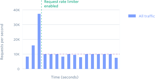
Image source: Stripe Blog
Leaky Bucket: Smoothing Traffic
The leaky bucket is conceptually the inverse of token bucket. Requests enter a queue (the bucket), and the system processes them at a fixed rate (the leak). If the queue is full, new requests are rejected.
This produces perfectly smooth output—exactly N requests per second, no bursts. For systems where downstream services can’t handle any variance in load, leaky bucket is the right choice.
The implementation typically uses a queue with a background process draining it at the configured rate. This introduces latency: requests sit in the queue until processed. For real-time APIs, this added latency may be unacceptable.
The critical difference from token bucket: leaky bucket strictly enforces average rate with no bursts. Token bucket allows temporary bursts up to the bucket capacity; leaky bucket forces all requests into a steady stream.
graph LR
    subgraph "Leaky Bucket"
        direction TB
        Queue[Request Queue]
        Leak[Fixed Rate Output]
    end

    R1[Request 1] --> Queue
    R2[Request 2] --> Queue
    R3[Request 3] --> Queue
    Queue -->|Process at N/sec| Leak
    Leak --> S[Smooth Output]

    style Queue fill:#e1f5fe
    style Leak fill:#c8e6c9
GCRA: The Elegant Algorithm from ATM Networks
The Generic Cell Rate Algorithm (GCRA) originated in Asynchronous Transfer Mode (ATM) networks—a technology largely forgotten but whose rate limiting innovation survives. GCRA achieves what leaky bucket does (smooth traffic, no bursts) with a single state variable instead of a queue.
GCRA tracks a theoretical arrival time (TAT)—the earliest time the next request is allowed. When a request arrives, calculate when the next request would be allowed if this one is accepted:
$$\text{TAT}_{\text{new}} = \max(\text{now}, \text{TAT}_{\text{old}}) + T$$Where T is the emission interval (1/rate). If the TAT is in the future, reject the request. Otherwise, update TAT and allow the request.
The algorithm also includes a tolerance parameter τ that allows limited bursting. A request arriving slightly before its ideal time is still allowed, but subsequent requests must wait longer. This provides some burst tolerance while preventing sustained over-rate traffic.
def allow_request(user_id, rate=10, tau=1.0):
    key = f"gcr:{user_id}"
    now = time.time()
    T = 1.0 / rate  # emission interval

    tat = redis.get(key) or now
    earliest = tat - T - tau  # earliest allowed time

    if now < earliest:
        return False  # too early

    new_tat = max(now, tat) + T
    redis.set(key, new_tat)
    return True
GCRA’s elegance is in its state efficiency. One timestamp per user, no queues, no background processes. The algorithm naturally smooths traffic while allowing controlled bursts. It’s particularly well-suited for distributed systems where minimizing state is critical.
Distributed Rate Limiting: The CAP Theorem Strikes
All the algorithms above assume a single rate limiter instance. In production, you likely have multiple instances across data centers. This introduces a fundamental challenge: consistency versus availability.
If you require perfect accuracy—every instance must have the same view of request counts—you need strong consistency. This means synchronizing state across instances before each request. The latency is unacceptable for most applications.
If you allow instances to operate independently—each maintaining its own counts—you sacrifice accuracy. A user could exceed their limit by hitting different instances. Cloudflare’s analysis showed this error is small (0.003%) but non-zero.
The CAP theorem frames this trade-off. Rate limiting systems typically choose AP (availability and partition tolerance) over CP (consistency and partition tolerance). During network partitions, the system continues operating with potentially inaccurate counts rather than failing entirely.
Redis Cluster makes this explicit. Data is sharded across nodes with replication. When a partition occurs, the cluster may accept writes on both sides—split brain from a consistency perspective, but available from an engineering perspective. For rate limiting, this is often acceptable: slightly inaccurate limits are better than denying all traffic.
Choosing the Right Algorithm
The algorithm you choose depends on what you’re protecting and what you’re willing to sacrifice:
Fixed Window Counter: Use when memory is constrained and occasional boundary bursts are acceptable. Best for coarse limits (daily API quotas) where precise timing doesn’t matter.
Sliding Window Log: Use when perfect accuracy is required and memory is abundant. Best for compliance requirements where every request must be accounted for.
Sliding Window Counter: Use when you need accuracy close to sliding window log but with minimal memory. This is the pragmatic choice for most web APIs.
Token Bucket: Use when users have legitimate burst patterns and you want to allow them. Best for developer-facing APIs where user experience matters.
Leaky Bucket: Use when downstream systems require perfectly smooth load. Best for rate-limiting writes to databases or external services with strict throughput requirements.
GCRA: Use when you want leaky bucket behavior without queue overhead. Best for distributed systems where state must be minimal.
The Production Reality
Rate limiting in production isn’t just about algorithms. Stripe documented four layers of rate limiting they deploy:
- Request rate limiter: Tokens per second per user
- Concurrent request limiter: In-flight requests per user
- Fleet usage load shedder: Reserve capacity for critical requests
- Worker utilization load shedder: Drop low-priority traffic when workers are saturated
The request rate limiter fires constantly—millions of rejections per month for misbehaving scripts. The worker utilization shedder fires rarely—only during major incidents. Each layer catches different failure modes.
This layered approach acknowledges a truth often missed in rate limiting discussions: no single algorithm solves all problems. Token bucket handles user-level fairness. Concurrent limits prevent resource exhaustion. Load shedders handle system-level emergencies. Together, they form a defense in depth.
The 2AM outage that opened this article had a simple fix: replace the fixed window counter with a sliding window counter. The boundary bursts stopped. The downstream services survived. But the deeper lesson is that rate limiting algorithm choice isn’t a minor implementation detail—it’s an architectural decision that determines how your system behaves under stress. Choose based on what you’re protecting and what you’re willing to sacrifice. There is no perfect solution, only appropriate trade-offs.
References
-
Cloudflare. (2017). “How we built rate limiting capable of scaling to millions of domains.” https://blog.cloudflare.com/counting-things-a-lot-of-different-things/
-
Stripe. (2017). “Scaling your API with rate limiters.” https://stripe.com/blog/rate-limiters
-
Brandur Lehn. (2015). “Rate Limiting, Cells, and GCRA.” https://brandur.org/rate-limiting
-
AlgoMaster. (2025). “Designing a Distributed Rate Limiter.” https://blog.algomaster.io/p/designing-a-distributed-rate-limiter
-
Arpit Bhayani. (2020). “Sliding Window Rate Limiting - Design and Implementation.” https://arpitbhayani.me/blogs/sliding-window-ratelimiter/
-
Zhang, Y., et al. (2026). “Designing Scalable Rate Limiting Systems: Algorithms, Architecture, and Distributed Solutions.” arXiv:2602.11741. https://arxiv.org/abs/2602.11741
-
Redis. (2026). “Build 5 Rate Limiters with Redis: Algorithm Comparison Guide.” https://redis.io/tutorials/howtos/ratelimiting/
-
GeeksforGeeks. (2026). “Rate Limiting Algorithms - System Design.” https://www.geeksforgeeks.org/system-design/rate-limiting-algorithms-system-design/
-
ByteByteGo. (2023). “Rate Limiting Fundamentals.” https://blog.bytebytego.com/p/rate-limiting-fundamentals
-
Kong. (2021). “How to Design a Scalable Rate Limiting Algorithm.” https://konghq.com/blog/engineering/how-to-design-a-scalable-rate-limiting-algorithm
-
ATM Forum. (1999). “Traffic Management Specification Version 4.1.” af-tm-0121.000. https://www.broadband-forum.org/download/af-tm-0121.000.pdf
-
Wikipedia. (2025). “Token bucket.” https://en.wikipedia.org/wiki/Token_bucket
-
Grab Tech. (2023). “Sliding window rate limits in distributed systems.” https://engineering.grab.com/frequency-capping
-
HikariCP Wiki. (2021). “About Pool Sizing.” (Referenced for distributed systems context)
-
Netflix. (2023). “concurrency-limits” GitHub Repository. https://github.com/Netflix/concurrency-limits