The Oracle Real-World Performance group published a demonstration that should have changed how every developer thinks about connection pools. They took a system struggling with ~100ms average response times and reduced those times to ~2ms—a 50x improvement. They didn’t add hardware. They didn’t rewrite queries. They reduced the connection pool size from 2048 connections down to 96.
Most developers configure connection pools based on intuition: more users means more connections, right? A typical production configuration sets the pool to 100, 200, or even 500 connections “just to be safe.” This intuition is precisely backwards. The correct question isn’t how to make your pool bigger—it’s how small you can make it while still handling your load.
What Actually Happens When You Open a Database Connection
Every database connection is expensive. Not just in the abstract sense, but in concrete, measurable resources that accumulate rapidly.
A PostgreSQL connection starts with a TCP handshake (one round-trip), then TLS negotiation if you’re connecting securely (two more round-trips for TLS 1.3, more for older versions), then authentication, then session initialization. For a client in New York connecting to a database in Singapore, that’s potentially 200-300ms before you’ve executed a single query. But even after the connection is established, the costs continue.
PostgreSQL uses a process-per-connection model. Each new connection triggers a fork() system call, creating a dedicated operating system process. AWS engineers measured the memory overhead of these connections in controlled tests. Freshly opened, idle connections consumed approximately 1.5 MB each. After running some queries—simulating normal application behavior—that number grew to 10-14 MB per connection. A thousand connections isn’t abstract: that’s 10-14 GB of RAM consumed just by having connections open, regardless of whether they’re doing anything.
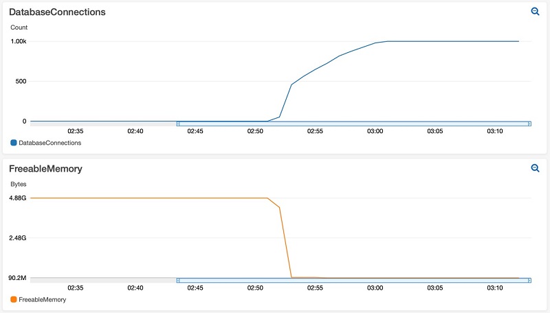
Image source: AWS Database Blog
The memory consumption isn’t just overhead. As connections eat into available RAM, the operating system has less room for filesystem cache. Database pages that would normally stay in memory get evicted. Queries that should complete in microseconds start hitting disk, taking milliseconds instead.
The Context Switching Problem
CPU cores can only execute one instruction at a time. When you have more active threads than cores, the operating system must perform context switches—saving the state of one thread, loading another, updating memory mappings, flushing and reloading CPU caches.
The cost of a context switch varies by system, but measurements typically show 1-10 microseconds of direct CPU overhead. The indirect costs are larger: the TLB (Translation Lookaside Buffer) that caches virtual-to-physical memory translations often gets flushed, causing subsequent memory accesses to be slower until the cache warms up again.
Here’s the brutal math: with 4 CPU cores and 100 active database connections, each core is juggling 25 connections. Even if each connection only needs 10 microseconds of CPU time per query, the context switching overhead accumulates rapidly. The CPU spends more time switching between connections than executing actual work.
graph LR
    subgraph "4 CPU Cores"
        C1[Core 1]
        C2[Core 2]
        C3[Core 3]
        C4[Core 4]
    end

    subgraph "100 Active Connections"
        direction TB
        G1[25 connections]
        G2[25 connections]
        G3[25 connections]
        G4[25 connections]
    end

    G1 -.->|Context Switch| C1
    G2 -.->|Context Switch| C2
    G3 -.->|Context Switch| C3
    G4 -.->|Context Switch| C4

    style G1 fill:#ff9999
    style G2 fill:#ff9999
    style G3 fill:#ff9999
    style G4 fill:#ff9999
The HikariCP project documented a PostgreSQL benchmark showing exactly this pattern. Throughput climbs as you add connections—up to a point. Then it plateaus. Add more connections beyond that peak, and throughput doesn’t just stop improving. It degrades.
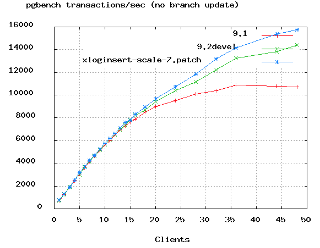
Image source: HikariCP Wiki
The chart shows TPS (transactions per second) flattening around 50 connections. The database in this test had 8 cores. The formula that emerges from this data, validated across years of benchmarks:
$$\text{connections} = (\text{core\_count} \times 2) + \text{effective\_spindle\_count}$$For an 8-core server with SSD storage (where spindle count is effectively zero), the optimal pool size is around 16 connections. Not 100. Not 200. Sixteen.
Why the Formula Works: Understanding I/O Wait
If CPU cores can only execute one thread at a time, why doesn’t optimal connection count equal core count? The answer lies in I/O wait.
When a query needs data that isn’t in memory, the database process blocks waiting for the disk. During that wait, it’s not using CPU. The operating system can execute another thread. Traditional spinning hard drives have seek times of 5-10 milliseconds—eternity in CPU time. With HDDs, having more threads than cores makes sense because threads spend significant time blocked on I/O.
SSDs change this equation. No moving parts means no seek time. I/O latency drops from milliseconds to microseconds. Less time blocked means fewer opportunities for other threads to use the CPU while waiting. The formula anticipates this: with SSDs, effective_spindle_count approaches zero, pushing the optimal connection count closer to core count.
This is counterintuitive but critical: faster storage means you should have fewer connections, not more. SSDs reduce blocking, which means less opportunity for context switching to provide value. Adding threads beyond the optimal point just adds overhead.
What AWS Discovered About Idle Connections
The assumption many teams make is that idle connections don’t matter. “Sure, we have 1000 connections open, but only 50 are active. The other 950 are just sitting there.”
AWS engineers tested this assumption rigorously. They ran pgbench against a PostgreSQL instance, measuring baseline transaction rates. Then they opened 1000 idle connections—connections that weren’t executing queries, just existing—and ran the same benchmark again.
The results were stark:
| Test Scenario | Without Idle Connections | With 1000 Idle Connections | Performance Impact |
|---|---|---|---|
| Standard pgbench | 1,249 TPS | 1,140 TPS | -8.7% |
| Select-only pgbench | 1,969 TPS | 1,610 TPS | -18.2% |
| Custom read-heavy query | 378 TPS | 206 TPS | -46% |
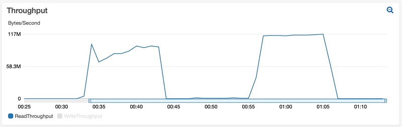
Image source: AWS Database Blog
The most dramatic case—a custom query reading 5000 rows per transaction—saw throughput cut almost in half. The idle connections weren’t doing work, but they were consuming memory that could have been used for cache. More disk reads, slower queries.
The Microservices Multiplication Problem
Connection pool sizing becomes exponentially harder in microservices architectures. Consider a typical setup:
- Database supports 200 maximum connections
- 10 microservice instances, each with its own connection pool
- Each instance configured with pool size of 20
That’s exactly 200 connections, right at the limit. But what happens during deployment? When rolling updates create old and new versions simultaneously? When auto-scaling kicks in during traffic spikes?
The math is unforgiving: if you scale to 15 instances, you’ve exceeded the database limit. Connection failures cascade. Timeouts propagate. What looked like adequate capacity becomes a production incident.
The solution requires coordination. If your database supports 200 connections and you might have 20 instances, each instance can only have a pool of 10. Not 20. Not “let’s set it to 20 just in case.” Ten. And you need monitoring to ensure the sum of all pools never exceeds the database capacity.
Connection Pool Modes: When Multiplexing Helps
External connection poolers like PgBouncer or cloud-managed proxies (AWS RDS Proxy) solve a different problem than application-level pools. They multiplex many client connections onto fewer database connections.
PgBouncer offers three modes:
Session pooling: Each client gets a dedicated database connection for the duration of its session. When the client disconnects, the connection returns to the pool. This provides compatibility with all PostgreSQL features but doesn’t help with idle connections—if a client is idle, its database connection sits idle too.
Transaction pooling: The database connection is only held during an active transaction. Between transactions, the client holds a lightweight connection to PgBouncer while the actual database connection serves other clients. This dramatically reduces database connection count for applications with significant idle time between queries.
Statement pooling: Even more aggressive—the connection can be reassigned between individual SQL statements. Maximum multiplexing, but breaks features that rely on session state (prepared statements, temporary tables, SET commands).
AWS tested transaction pooling against the same workload that showed 46% degradation with idle connections. With PgBouncer configured for 20 database connections handling 1000 client connections, performance remained stable. The idle clients held connections to PgBouncer, not to PostgreSQL itself. The database saw only active work.
sequenceDiagram
    participant App1 as Application Instance 1
    participant App2 as Application Instance 2
    participant Pooler as Connection Pooler
    participant DB as Database

    Note over Pooler: Pool maintains 20 DB connections

    App1->>Pooler: Request connection
    Pooler->>DB: Use connection from pool
    App1->>Pooler: Execute transaction
    Pooler->>DB: Forward query
    DB-->>Pooler: Results
    Pooler-->>App1: Return results
    App1->>Pooler: Release connection
    Note over Pooler: Connection returns to pool

    App2->>Pooler: Request connection
    Note over Pooler: Same DB connection reused
    Pooler->>DB: Use connection from pool
Calculating Your Pool Size
The formula $(core\_count \times 2) + effective\_spindle\_count$ provides a starting point, not an absolute answer. Real optimization requires understanding your workload:
CPU-bound queries (complex joins, aggregations, in-memory operations): Stay closer to core count. Queries are using CPU continuously, so additional connections just create context switching overhead.
I/O-bound queries (table scans on uncached data, heavy writes): More connections can help, as threads waiting on I/O create opportunities for others to execute. But measure—modern SSDs blur this line.
Mixed workloads (the common case): This is where two-pool strategies help. A small pool for latency-sensitive queries, a larger pool for batch operations. The two don’t interfere with each other.
A practical approach:
- Start with the formula
- Run load tests at expected traffic levels
- Monitor: connection wait time, query latency, CPU utilization
- If connections are waiting for the pool, increase slowly
- If CPU is saturated but connections are waiting, the database is the bottleneck—adding connections won’t help
- If latency increases under load with available connections, you may have passed the optimal point
The Monitoring That Matters
Connection pool misconfiguration manifests in specific ways:
-
Pool exhaustion: Threads waiting for connections. Look for spikes in
HikariPool-1 - Connection is not availableerrors or equivalent for your pooler. The fix isn’t always more connections—often it’s faster queries or better transaction management. -
High context switch rate: On Linux,
pidstat -w 1shows context switches per second. A database server with single-digit cores and thousands of context switches per second is spending more time switching than working. -
Cache hit rate degradation: PostgreSQL’s
pg_statio_user_tablesshows buffer hits versus disk reads. If hit rates drop as connection count rises, connections are consuming memory that should be cache. -
Lock contention: More connections mean more potential for lock conflicts. Monitor
pg_locksand lock wait events. Sometimes the “solution” to lock contention is fewer connections, not more.
When More Connections Are Actually the Answer
Not every situation calls for minimal pools. There are legitimate reasons to increase:
Long-running transactions: A connection held for 30 seconds for a batch job reduces available connections for OLTP queries. If you can’t eliminate the long transactions, you may need additional connections to maintain OLTP throughput. Better: isolate long-running work to separate pools or even separate databases.
Connection acquisition overhead: If your application rapidly opens and closes connections (an anti-pattern, but common in serverless environments), you might see connection establishment as a significant portion of latency. The fix is usually better connection management, but sometimes a larger pool smooths over burst behavior.
External constraints: Some ORMs and frameworks open multiple connections per thread. If your application architecture requires three connections per worker thread and you have 20 threads, you need at least 60 connections. The deadlock-prevention formula gives: $\text{pool\_size} = T_n \times (C_m - 1) + 1$, where $T_n$ is threads and $C_m$ is max connections per thread.
Summary of Principles
The counterintuitive truth about connection pools:
-
Smaller is usually better: The optimal pool size is typically $(cores \times 2)$, not hundreds of connections.
-
Idle connections aren’t free: They consume memory, reduce cache, and can degrade performance by 8-46% even while doing no work.
-
SSDs change the equation: With faster storage, optimal connection counts approach core count.
-
Microservices multiply the problem: Coordinate pool sizes across all instances to stay within database limits.
-
Poolers help at the cost of features: Transaction pooling dramatically reduces database connections but breaks session-level PostgreSQL features.
-
Context switching is overhead, not progress: More threads than cores means time spent switching rather than executing.
-
The formula is a starting point: Measure your workload. The right size depends on your specific query patterns, hardware, and latency requirements.
The next time you see a connection pool configured to 100 or 200 “just to be safe,” consider: you might be configuring yourself into a performance problem. The Oracle Real-World Performance group demonstrated a 50x latency improvement from reducing pool size. The fix might be that simple.
References
-
HikariCP Wiki. “About Pool Sizing.” GitHub, 2021. https://github.com/brettwooldridge/HikariCP/wiki/About-Pool-Sizing
-
Raja, Yaser. “Resources Consumed by Idle PostgreSQL Connections.” AWS Database Blog, 2021. https://aws.amazon.com/blogs/database/resources-consumed-by-idle-postgresql-connections/
-
Raja, Yaser. “Performance Impact of Idle PostgreSQL Connections.” AWS Database Blog, 2021. https://aws.amazon.com/blogs/database/performance-impact-of-idle-postgresql-connections/
-
Schneider, Andres. “Analyzing the Limits of Connection Scalability in Postgres.” Microsoft Tech Community, 2020. https://techcommunity.microsoft.com/blog/adforpostgresql/analyzing-the-limits-of-connection-scalability-in-postgres/1757266
-
PgBouncer Documentation. “Features.” https://www.pgbouncer.org/features.html
-
MySQL Documentation. “MySQL Connection Handling and Scaling.” Oracle, 2019. https://dev.mysql.com/blog-archive/mysql-connection-handling-and-scaling/
-
Little, John D. C. “A Proof for the Queuing Formula: L = λW.” Operations Research, vol. 9, no. 3, 1961, pp. 383-387.